User-friendly p-values
Posted by Joachim Goedhart, on 13 February 2019
A good statistic is the one that you can understand. Mean values are understandable and everybody knows how to calculate them. Most people also realize how the mean value can be skewed by an outlier. So we know what the mean represents and we are aware of its limitations. In sharp contrast, the Null Hypothesis Significance Test (NHST) and the resulting p-values are poorly understood. Although there is nothing wrong with the p-value itself, its calculation and interpretation are far from intuitive (Greenland et al., 2016).
The backward logic of the p-value contributes to its poor understanding (footnote 1). It doesn’t help that the calculation of p-values is usually done with a piece of software, without knowing and understanding the underlying calculation. Notwithstanding these issues, the calculation and reporting of p-values is a standard practice. I think it is very ironic that p-values are widely used and at the same time poorly understood. Since it is unlikely that p-values will disappear any time soon, a user-friendly, understandable calculation of p-values would be very helpful. Below, I will explain a method for calculating a p-value that I find much easier to understand. This method is known as the (approximate) permutation or randomization test. There are also some excellent explanations of this method by others (Hooton, 1991; Nuzzo, 2017).
Before we start: conditions and assumptions
I will deal with the randomization test and treat the case where data is sampled from two independent conditions. The requirements for this test are not different from any other statistical significance test. The data of the samples needs to be random, independent and representative of the population that it was sampled from. A convenient aspect of the randomization test is that it makes no assumption with respect of the data distribution. So, it does not require the data to adhere to a normal distribution (in contrast to the Student’s t-test or Welch’s t-test).
Example data
I will explain the randomization test with experimental data obtained in our lab (and previously used to explain the calculation of the effect size). There is a “Control” condition (n=74) and a “TIAM” condition (n=110) for which the cell area is determined. These two conditions will be compared in the randomization test.
The null hypothesis
The null hypothesis states that there is no difference between the mean of the reference (“Control”) and mean of the treated (“TIAM”) condition. For the randomization method, we rephrase the null hypothesis: All the observed data is sampled from the same population. As a consequence, there is no difference between the mean value of the two conditions. Note that this rephrased null hypothesis is essentially the same as the classical null hypothesis.
The randomization method
The procedure is broken down in 5 steps. Each step is shown in figure 1 and explained below.
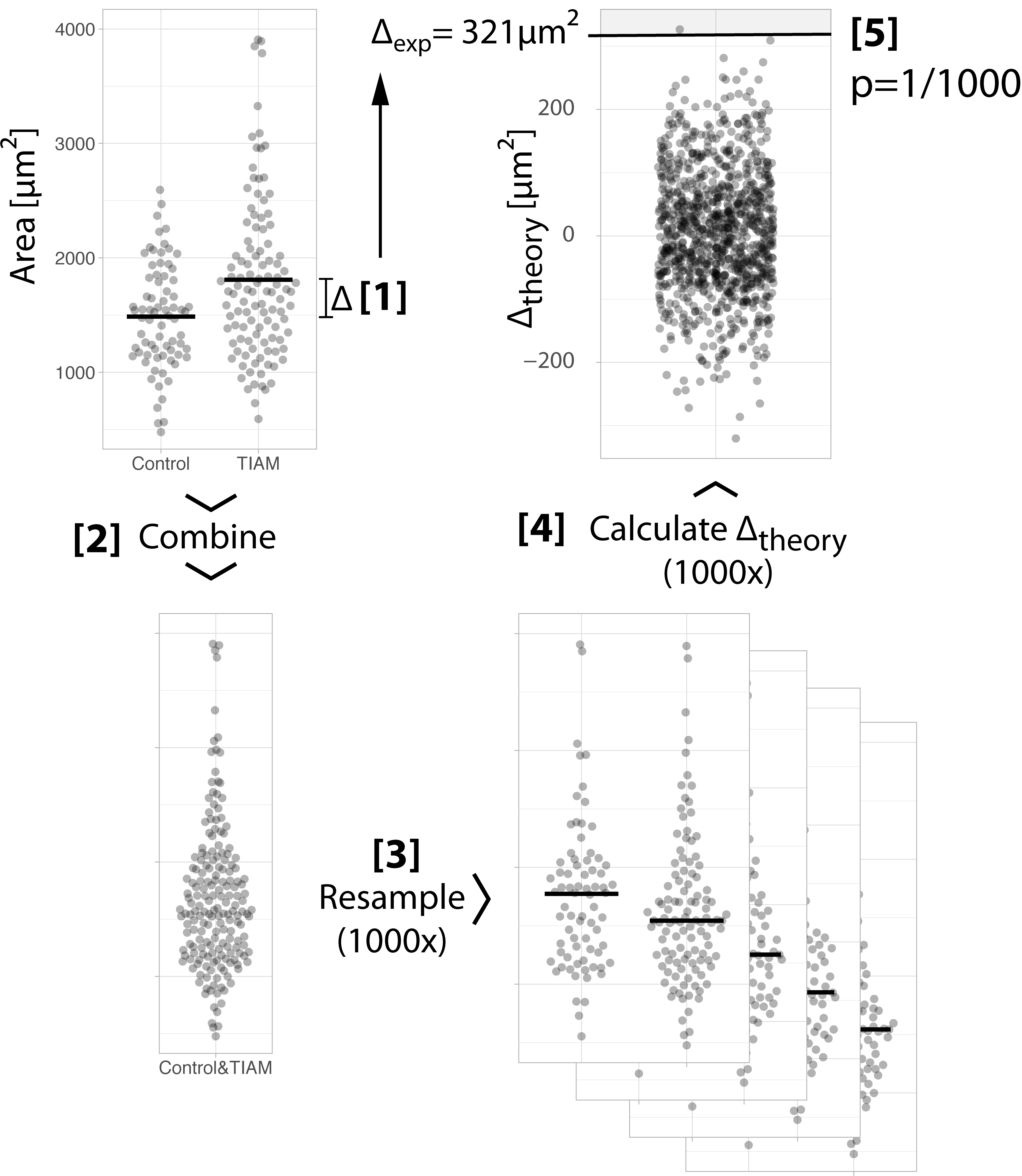
Figure 1: Step-by-step explanation of the randomization method. Each of the steps is explained in the main text.
Step 1: We calculate the difference between the mean of the two conditions: 1808-1487=321 µm². This is the ‘observed difference’ between the means.
Step 2: We combine the data of both conditions to generate a single aggregated sample. We put all data together because the null hypothesis states that all data was sampled from this distribution.
Step 3: We draw two random samples from the aggregated sample (the samples have the same size as the original control and treated samples, i.e. n=74 and n=110 respectively). This is repeated many times, typically 1000x.
Step 4: For every single new sample, we calculate the difference between the means. This is a ‘theoretical difference’, since it is a difference that could arise when the samples were obtained from the same population. We end up with a collection of 1000 theoretical differences. The distribution of the theoretical differences is also known as the null distribution. In summary, we have constructed a distribution of theoretical differences that could have been observed when all data came from one and the same population.
Step 5: We compare the observed difference between the means from step 1 with the null distribution that we generated in step 4. This comparison is the same as asking: “How likely is our observed difference (or more extreme differences), given that the data were sampled from the same population?”. We see in figure 1 that the observed difference is quite different from the theoretical differences. In fact, only 1 out of 1000 theoretical differences exceeds the observed difference. Therefore, the probability of our observed difference between the means (or more extreme differences) given that the data are sampled from the same population is 1/000. This probability, or p-value, of 0.001 tells us that we have a rather extreme observation and it provides strong ground for rejecting the null hypothesis.
Beyond the mean
The mean may not be the best measure of centrality due to its sensitivity to outliers. The example data used here seems asymmetric and it that case the median is a better measure of centrality. Consequently, we may be more interested in differences between median values. Luckily, the randomization test is readily adapted to examine a difference in medians (Hooton, 1991). We can repeat the entire procedure for the difference between medians (figure 2). First, the difference in the experimental data is 196 µm². Next, we resample the combined data and calculate the difference in medians for each of the sample. The resulting null distribution is compared with the experimentally observed difference in medians. It shows that the probability of the observation (or more extreme values) is 17 out of 1000. The p-value for the difference in medians is 0.017.
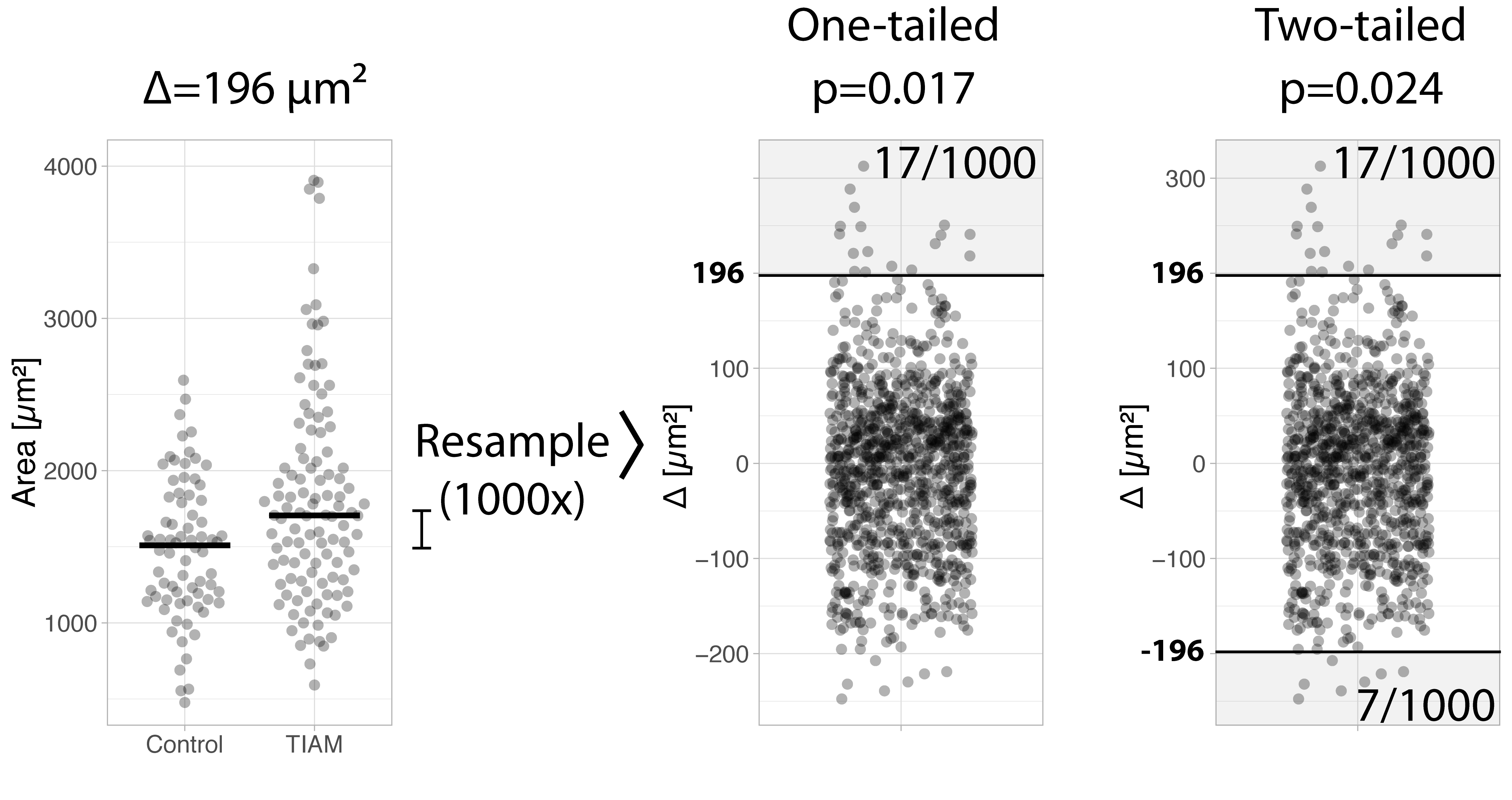
Figure 2: Example of a randomization test for comparing medians, explaining the one-tailed and two-tailed comparison
The devil is in the (de)tails
So far, we have only considered one side of the null distribution. This is known as a one-tailed test. However, we are often interested in finding any difference and we do not consider the directionality. In other words, we are looking for a difference that can be either positive or negative. This is known as a two-tailed test. For a two-tailed test we consider both tails for the difference of medians. We find that in the other tail of the null distribution there are 7 (theoretical) values more extreme than our observed value of 196 µm². Therefore the p-value for the two-tailed test is p=(17+7)/1000=0.024 (figure 2, right panel). Based on this p-value we can reject the null hypothesis and conclude that the two samples do not originate from the same population.
Final words
Like any other statistical test, the permutation and randomization methods are not without limitations or shortcomings (Wilcox and Rousselet, 2018). And regardless of the way a p-value is calculated, it is recommended to supplement p-values with other statistical parameters (Wasserstein and Lazar, 2016). A good alternative for p-values is the calculation of the effect size, because it quantifies the magnitude of the difference. To me, the rather straightforward calculation and more intuitive determination of a p-value by the randomization method is a big advantage over classical null hypothesis tests. Possibly the biggest benefit is that this method makes it clear that we determine the probability of the data in relation to the null hypothesis (instead of determining the probability that the null hypothesis is true as is often mistakingly thought, see also Footnote 1). The randomization method is also well suited for teaching and examining the properties of p-values. To conclude, I hope that the user-friendly p-value will aid in understanding null hypothesis testing and also help in recognizing the limitations of p-values.
DIY
The data and R-script to perform the randomization method is avaliable at Zenodo: http://doi.org/10.5281/zenodo.2553850
A web-based application that calculates p-values by randomization is currently under development and available: http://huygens.science.uva.nl/PlotsOfDifferences/
The source code for the web tool is on GitHub: https://github.com/JoachimGoedhart/PlotsOfDifferences
Footnotes
Footnote 1: The p-value is the probability of the data (or more extreme values) given that the null hypothesis is true. However, its definition is often mistakingly(!) flipped and taken as a probability that the null hypothesis is true (Greenland et al., 2016).
 (16 votes)
One thought on “User-friendly p-values”
Leave a Reply
Get involved
Create an account or log in to post your story on the Node.
Sign up for emails
Subscribe to our mailing lists.
Note that Andrew Plested has python code available to run the randomization test: https://github.com/aplested/DC-Stats