Make a difference: the alternative for p-values
Posted by Joachim Goedhart, on 8 October 2018
Calculation and reporting of p-values is common in scientific publications and presentations (Cristea and Ioannidis, 2018). Usually, the p-value is calculated to decide whether two conditions, e.g. control and treatment, are different. Although a p-value can flag differences, it cannot quantify the difference itself (footnote 1). Therefore, p-values fail to answer a very relevant question: “How large is the difference between the conditions?” (Gardner and Altman, 1986; Cumming, 2014). The aforementioned question can be answered by calculating the “effect size”, which quantifies differences. Calculation and interpretation of effect sizes is straightforward and therefore a good alternative for calculating p-values (Ho, 2018). In the figure below, I transformed an ordinary plot with p-values into graphs that depict (i) the data and (ii) the difference between median values as the effect size. The calculation and application of effect sizes is the topic of this blog.
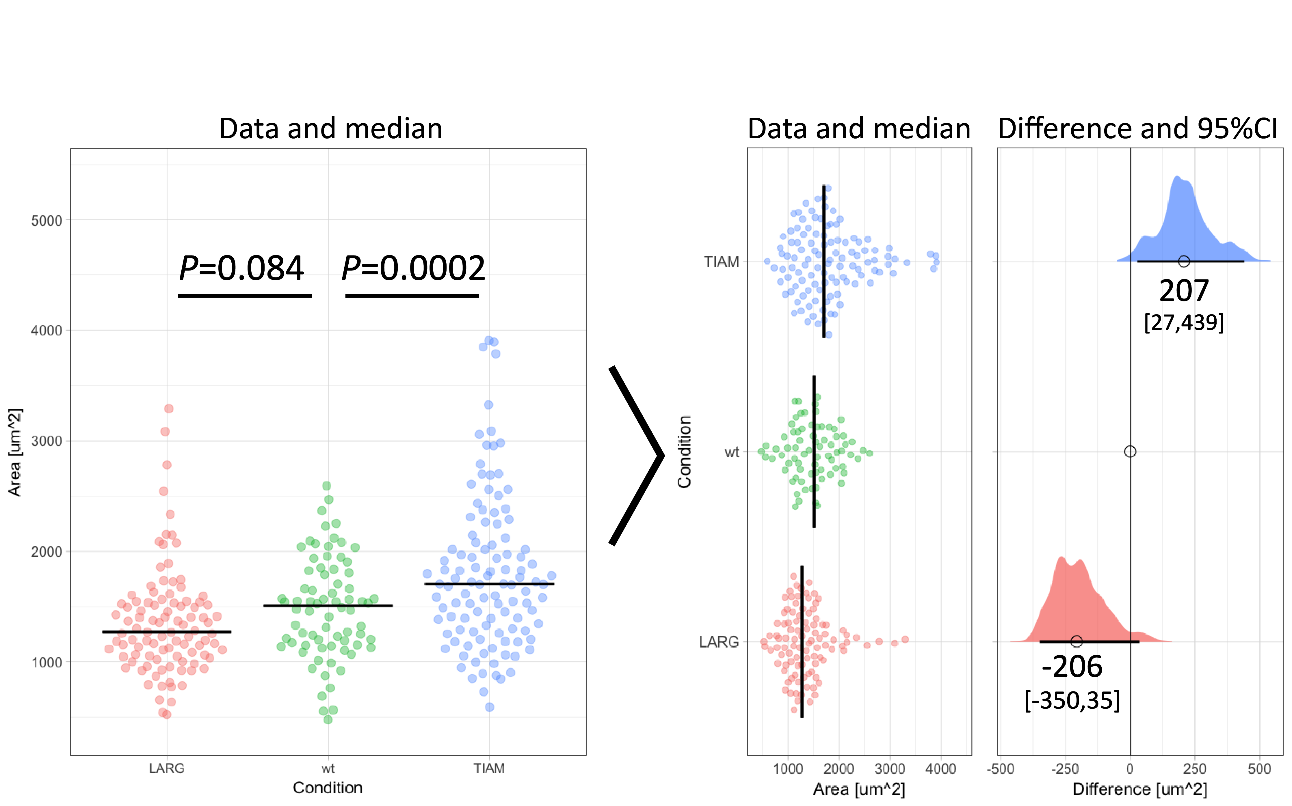
Figure 1: Transformation of an ordinary graph with p-values into a visualization of the data and the difference between median values as the effect size. Values indicate the difference between the median and the median of the ‘wt’ Condition. The horizontal lines and the values between brackets indicate the 95% confidence interval.
Why do we need an alternative for p-values?
The null-hypothesis significance test (NHST) compares the central tendency of two samples, e.g. the mean for parametric or median for nonparametric tests. Next to the central tendency (or location), it takes into account the precision of that value. Since the precision increases with increasing sample size, the outcome of a NHST depends on sample size (Nakagawa and Cuthill, 2007) as also explained here. In other words, the p-value reflects both the difference in central tendency and the number of observations. This is just one of the issues with p-values, other issues that should be considered when using p-values are discussed elsewhere (Goodman, 2008). Due to the issues with p-values, it has been recommended to replace (Cumming, 2014; Halsey et al., 2015) or supplement (Wasserstein and Lazar, 2016) p-values with alternative statistics. Effect sizes, aka estimation statistics, are a good alternative (Claridge-Chang and Assam, 2016).
Effect size
In statistics, the effect size reflects the difference between conditions. In contrast with p-values the effect size is independent of sample size. Effect sizes are expressed as relative (footnote 2) or absolute values. Here, I will only discuss the absolute effect size. The absolute effect size is the difference between central tendency of samples. Commonly used measures of central tendency are the mean and median for normal and skewed distributions respectively. Hence, for a normal distribution the effect size is the difference between the two means.
Quantification of differences
To illustrate the calculation and use of effect sizes, I will use data from an experiment in which the area of individual cells was measured under three conditions (Figure 1). There is an untreated (wt) condition and two treated samples. The question is how the treatment affects the cell area. When the distribution of the observed areas is non-normal (as is the case here), the median better reflects the central tendency (i.e. typical value) of the sample. Therefore, it is more adequate for this experiment to calculate the difference between the medians (Wilcox, 2010). The median values for TIAM, wt and LARG are 1705 µm², 1509 µm² and 1271 µm² respectively. From these numbers, it follows that the effect of TIAM is an increase of area by 1705 µm² – 1509 µm² = 196 µm². The effect of LARG is a decrease in cell area of 1271 µm² – 1509 µm² = -238 µm². Note that the difference is expressed in the same units (e.g. µm²) as the original measurement and is therefore easy to understand.
Confidence intervals
As mentioned before, the difference will not depend on sample size. On the other hand, the precision will depend on sample size. More observation per experimental condition will generate median values with a lower error. As a consequence, the difference will be more precisely defined with a larger sample size (Drummond and Tom, 2011). To indicate the precision of the difference, the 95% confidence interval (95CI) is a suitable measure (Cumming, 2014). For differences between means, the 95CI can be calculated directly (see here or here for calculation with R) but for the difference between medians it is not straightforward.
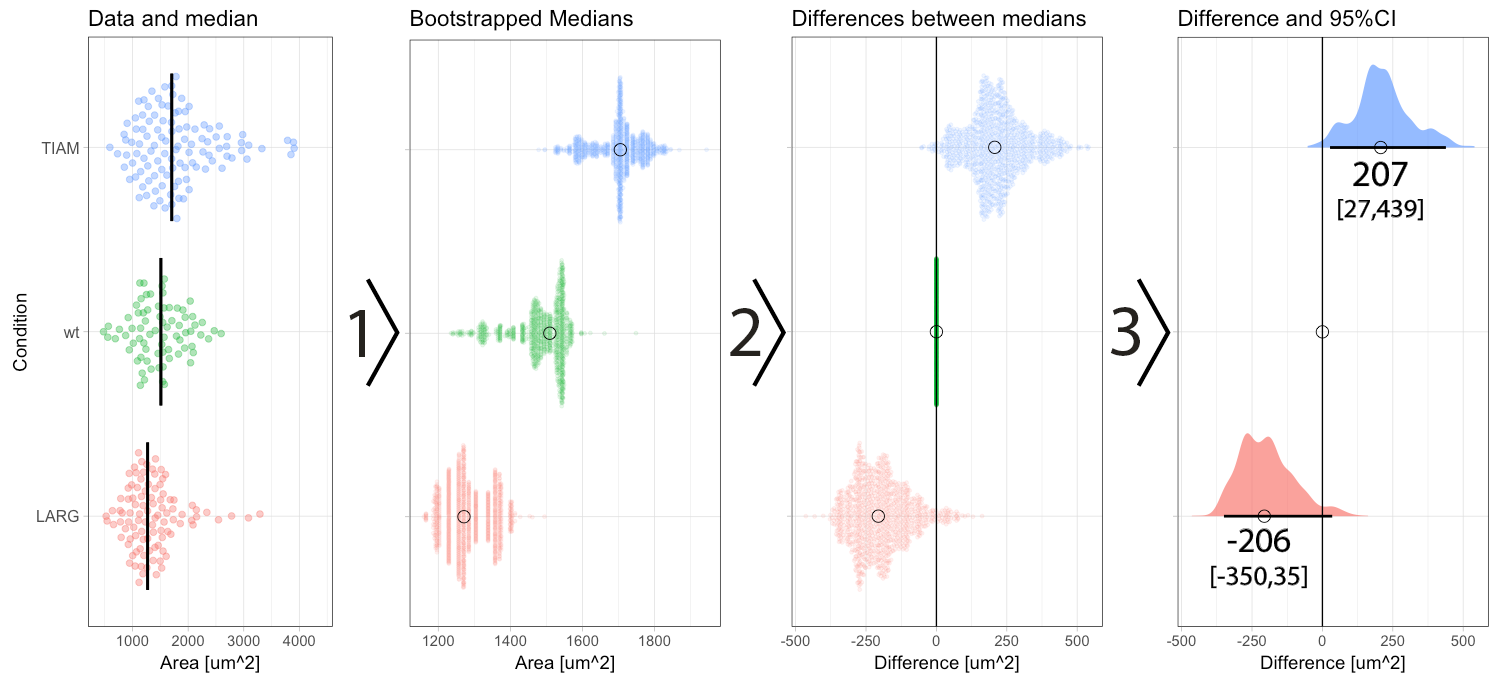
Figure 2: Step-by-step explanation of the calculation and visualization of the effect size and 95% confidence intervals. Step 1) bootstrapping of the data results in a collection of 1000 new median values. Step 2) the difference between the conditions (LARG and TIAM) and the control (wt) is calculated by subtraction, yielding 1000 differences (or effect sizes). Step 3) the middle value (median) of the distribution defines the effect size and the borders encompassing 95% of the differences define the 95% confidence interval (95CI, values between brackets). Medians are indicated with a circle and the 95CI with a horizontal line.
Median difference with confidence intervals
In a previous blog, I explained how bootstrapping can be used derive the 95CI of the median. Briefly, bootstrapping is resampling of existing data in silico, typically 1000 times. This process simulates repeating the actual experiment (footnote 3). Bootstrapping can be done with the data of the experiment, for each of the conditions, yielding 1000 median values which are displayed in figure 2 (step 1). The 1000 medians reflect a distribution of values that would have been obtained, if the experiment were to be repeated 1000x. These bootstrapped medians can be used to calculate the effect size, i.e. difference between the median of the control group and the other conditions. The result of the calculation is 1000 difference values per condition (figure 2, step 2). The resulting distribution of the differences can be used to determine the 95CI. As explained previously, the 95CI is taken from the middle 95% of the data, i.e. the values at the 2.5th and 97.5th percentile (figure 2, step 3). Thus, by bootstrapping we obtain the difference between medians and the 95CI (footnote 4).
Result and interpretation
The resulting graph shows two effect sizes with confidence intervals. All values are in the original units (µm²) and therefore these numbers make sense. The effect of TIAM is an area change of 207 µm² with a 95CI that ranges from 27 µm² to 439 µm² (footnote 5). The confidence interval can be listed between brackets: [27,439]. Since the 95CI does not overlap with zero (as also clear from the graph in figure 1 and 2), this is interpreted as a significant change (at an alpha level of 0.05). On the other hand, the effect of LARG is -206 [-350,35] µm². Since the 95CI does overlap with zero for this condition, this implies that there is no conclusive evidence for an effect. Note that the interpretation of the confidence intervals is consistent with the p-values listed in figure 1. For more information on the interpretation of effect size and 95CI see table 5.2 by Yatano (2016).
Conclusion
The effect size is the difference between conditions. It is of great value for the quantitative comparison of data and it is sample size independent. Another advantage is that the effect size is easy to understand (in contrast to p-values, which are often misunderstood or misinterpreted). The benefit of the bootstrap procedure to derive the confidence intervals is that it delivers a distribution of differences. The distribution conveys a message of variability and uncertainty, reducing binary thinking. So, make a difference by adding the effect size to your graph. The effect size facilitates interpretation and can supplement or replace p-values.
Acknowledgments: Thanks to Franka van der Linden and Eike Mahlandt for their comments.
Availability of data and code
The data and R-script to prepare the figures is available at Zenodo: https://doi.org/10.5281/zenodo.1421371
A web-based application (using R/ggplot2) for calculating and displaying effect sizes and 95CI (based on bootstrapping) is currently under development: https://github.com/JoachimGoedhart/PlotsOfDifferences
A preview of the web app is available here.
Footnotes
Footnote 1: The actual definition of a p-value is: The probability of the data (or more extreme values) given that (all) the assumptions of the null hypothesis are true.
Footnote 2: Examples of relative effect size are Cohen’s d and Cliff’s delta. The Cliff’s delta is distribution independent (i.e. robust to outliers) and can be calculated using an excel macro, see: Goedhart (2016)
Footnote 3: Bootstrapping assumes that the sample accurately reflects the original population that was sampled. In other words, it assumes that the sampling was random and that the samples are independent. These assumptions also apply to other inferential statistics, i.e. significance tests.
Footnote 4: The website www.estimationstats.com (developed by Adam Claridge-Chang and Joses Ho) uses bootstrapping to calculate the effect size and 95CI for the difference of means. It is also a good source for information on effect sizes.
Footnote 5: Bootstrapping depends on random resampling, and therefore the numbers will be slightly different each time that resampling is performed.
 (20 votes)
4 thoughts on “Make a difference: the alternative for p-values”
Leave a Reply
Get involved
Create an account or log in to post your story on the Node.
Sign up for emails
Subscribe to our mailing lists.
I think the things mentioned are good if we have paired data. If the data is not dependent, then we cannot do any of the things mentioned. Anyway, it was a good read. Thanks for the post
In case of paired data, it is possible to directly calculate the difference. Here, for independent data, the difference between the means (or medians) of two samples is calculated. This can be done (and is straightforward) – it’s a bit more complex if one wants to calculate the precision/uncertainty
The web tool ‘PlotsOfDifferences’ is described in a preprint: http://biorxiv.org/cgi/content/short/578575v1
Very cool. I came up with the same approach and now am applying it for writing a scientific article. Yet, I wonder why this approach has not been widely recognized/used till now…
I guess there is no very famous name on this, like “t-test”, and very few references can be found. Correct me if wrong. I would appreciate if anyone can share the first article that suggested this approach (or, is this blog the first one?).