The Collaborative Research Centre 1348 “Dynamic Cellular Interfaces: Formation and Function” at the University of Münster, Germany, invites applications for
10 PhD Positions
(salary level E13 TV-L, 65%)
Projects are available from the earliest possible date for three years. Currently, the regular full employment time is 39 hours and 50 minutes per week.
The Collaborative Research Center 1348 uses an integrated research approach to investigate the formation and function of dynamic cellular interfaces, which are the basis for many biological processes ranging from cellular differentiation to synapse function and maintenance. CRC1348 provides a stimulating, interdisciplinary, international research environment with 20 participating groups from three faculties at the University of Münster and the Max Planck Institute of Molecular Biomedicine. Within CRC 1348, the Integrated Research Training Group (IRTG) offers a structured doctoral programme, including a supervision concept, measures for career development, as well as a tailored training programme with subject-based interdisciplinary research and soft skills courses. Support with administrative matters, accommodation and visas are part of the program.
PhD projects involve state-of-the-art imaging as well as molecular, genetic and biochemical approaches. Projects are available in the areas of cell and developmental biology, neurobiology, vascular biology, virology, biophysics and physical chemistry. For details about the projects, please see http://sfb1348.uni-muenster.de/projects.
We invite applications from highly qualified and motivated students of any nationality with a strong background in life sciences or biomedicine. A master’s or equivalent degree in biology, biochemistry or a related field is required. Applications from candidates interested in quantitative imaging and biophysical approaches are especially welcome. Applicants are expected to show a high level of proficiency in both spoken and written English. German language skills are not required.
The University of Münster is an equal opportunity employer and is committed to increasing the proportion of women academics. Consequently, we actively encourage applications by women. Female candidates with equivalent qualifications and academic achievements will be preferentially considered within the framework of the legal possibilities. We also welcome applications from candidates with severe disabilities. Disabled candidates with equivalent qualifications will be preferentially considered.
Application documents should include a curriculum vitae, a grade transcript and a motivation letter. Applicants should state their scientific interests in one or more of the specific CRC projects. Additionally, applicants should arrange for two letters of recommendation to be submitted directly to applications.crc1348@uni-muenster.de
Transportation networks play a central role in enabling efficient mass flow over extended domains, where diffusion alone would be too slow. Therefore, transportation networks often play a central role for an organism’s physiology and a high degree of energetic efficiency has been proposed as a guiding principle for the layouts of these networks.
However, biological organisms usually do not construct their networks only after fully developing the body plan, but instead extend them together with the growth of the body, for example in trees, fungi, or myxomycetes. Then it is interesting to ask how they achieve a high degree of efficiency, given that at the time of network construction the final shape of the organism is yet unknown.
Physarum polycephalum: a Crawling Network
Figure 1: Physarum polycephalum in a near-natural environment in a terrarium. Note the fan-like structures that are extension fronts emerging from a multitude of connected veins.
The true slime mould Physarum polycephalum (see fig. 1) is a good model for this question, for two reasons. First, it is an easy-to-handle, macroscopic organism that prominently features an adaptive tube network as it extends over surfaces.More importantly, though, we have an understanding of the rules that shape this network under static conditions: a simple set of equations formulated by Tero et al. (J. Theor. Biol. 2007) known as the ‘current reinforcement rule’.
To learn how network formation occurs during extension, it makes sense to first study the organism’s behaviour under this condition and then find a model that explains this behaviour. A model enables us to make testable predictions that can decide whether we have, in fact, understood the basic characteristics of the organism and to include certain assumptions about the mechanism behind them.
Study Approach: Learn, Model, Check
1. Learn
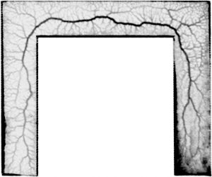
Figure 2: Physarum polycephalum having just explored a 5mm-wide lane from the bottom left to the bottom right. Note the development of a central main vein tracing a centre-in-centre trajectory at both turns of the lane.
In a study published last year (Schenz et al.,J. Phys. D 2017), we first studied how the network of Physarum under extension is shaped. We let the organism extend through a narrow lane that includes some turns (see fig. 2). The organism constructed its main veins at a small distance behind the growth front and did so at a time long before it had fully explored the complete layout of the arena. The main characteristic of the resultant vein trajectory is that it cuts corners at turns but then returns back to the centre line of the arena, even between two turns, where the globally shortest path would dictate to remain on the inside edge.
Nevertheless, analysis showed that the slime mould’s main vein was only 6% longer than the shortest possible route through the arena. To appreciate this, one has to consider that a naïve strategy of constructing the vein in the centre of the corridor would result in a trajectory 18% longer than the minimum. How can we explain such a high efficiency in the absence of foresight?
2. Model
As a model we considered first the classical current reinforcement model, but it failed to reproduce the characteristic vein pattern. Therefore, current reinforcement dynamics alone are insufficient to explain the organism’s capability. As a consequence we constructed a novel model consisting of three core elements that have each been successfully used in the literature to describe specific aspects of Physarum physiology: wave front dynamics, Calcium-driven oscillation waves, and the current reinforcement tube model. We linked these three elements with appropriate interactions under the assumption that the observed expansion behaviour and network structure are a consequence of their interplay.
The resulting model explained the phenotypical features well both qualitatively and quantitatively, and also contained some physiological assumptions that are testable. We could thus determine that the coupling between growth front extension and tube network evolution has to be of just the right strength to allow the organism some spatial integration necessary to find local optimality of the route trajectory as well as efficient transportation of body mass through the tube network from the rear to the front.
3. Check
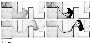
Figure 3: A comparison between the actual vein trajectory (left) and the same pictures as on the left but overlaid with vein predictions based on our algorithm (right).
The corollary of this finding is that growth front extension history alone should be sufficient to make a prediction on the main vein trajectory (see fig. 3). This hypothesis yielded much better predictions than alternative explanations we tested. This then yields a mechanistic explanation of how the organism can achieve this high degree of optimality in the face of uncertainty and at the same time an interpretation for the biological context for the current reinforcement rule: to enable efficient locomotion of Physarum.
In our ongoing research we develop further the question of what measure of optimality is likely guiding an expanding network. Total network length, as considered above, is not the only dimension along which a network can be evaluated, especially if it is embedded in a foraging organism. We will, therefore, search for such a measure that best predicts the behaviour of the organism given greater degrees of freedom to then evaluate well established concepts such as Optimal Foraging Theory in the context of continuous, network-based systems. This will allow us to consider how efficient networks have to be structured in an unknown environment.
Venue: St. John’s College, University of Oxford, Oxford, UK
Dates: 23-25 July 2018
Many human psychiatric and neurological conditions have developmental origins. Rodent models are extremely valuable for the investigation of brain development, but cannot provide insight into aspects that are specifically human. The human cerebral cortex has some unique genetic, molecular, cellular and anatomical features which need to be further explored. At the winter meeting of the Anatomical Society in 2010 we hosted a symposium focussed on development of the human cerebral cortex cortex. At that time a renaissance in the study of human brain development was getting underway made possible by the availability of new techniques, such as generation of human neural stem cells and organoids ex vivo, in utero MRI, and RNAseq and resources such as the Human Developmental Biology Resource and the Allen Brain Atlas. Eight years later, we feel the time has come to review the spectacular progress made since the last meeting. An international cast of speakers will provide insights into the cellular and molecular features of human cortical expansion and evolution, uniquely human features of cortical circuit formation, the development of the subplate in health and disease, and the origins of human cortical malformations, amongst other topics. We look forward to welcoming you to St John’s College for this exciting event.
Invited Speakers
Andre Goffinet, Bruxelles
Arnold Kriegstein, San Francisco
Bruno Mota, Rio de Janeiro
Charles Newton, Oxford
David Edwards, London
Eleonora Aronica, Amsterdam
Eva Anton, Chapel Hill
Fiona Francis, Paris
Gavin John Clowry, Newcastle
István Adorjan, Budapest
Ivica Kostovic, Zagreb
James Bourne, Melbourne
Kjeld Møllgård, Copenhagen
Mary Rutherford, London
Milos Judas, Zagreb
Nenad Sestan, New Haven
Pasko Rakic, New Haven
Patricia Garcez, Rio de Janeiro
Petra Hüppi, Geneva
Robert Hevner, Seattle
Susan Lindsay, Newcastle
Trygve Bakken, Seattle
Xiaoqun Wang, Beijing
Zoltan Molnar, Oxford
Voting has just closed, and with precisely 800 votes counted, we can now reveal the top three –
3rd Place (17% of the votes)
Sea anemone by Maria Belen Palacios
2nd Place (26% of the votes)
Drosophila by Eugene Tine
1st Place (36% of the votes)
Drosophila by Soraya Villaseca
Blue: DAPI, green: motor neuron axons, pink: motor neuron nuclei
Congratulations to Soraya, and thanks to the other competitors Maria Belen Palacios, Eugene Tine, Luiza Saad and Estefanía Sánchez Vásquez. Look out for Soraya’s image on a Developmentcover later this year!
preLights, The Company of Biologist’s new preprint highlighting service, has now been running for more than three months. At the heart of preLights is the community of early-career researchers who select and highlight interesting preprints in various fields.
The preLights banner features cultured rat hippocampal neurons from Christophe Leterrier
We are now ready to grow our team of preLighters and are seeking early-career researchers, who are passionate about preprints and enjoy writing and communicating science. We welcome scientists across the biological sciences and especially those with expertise in Neuroscience, Bioinformatics, Microbiology, Ecology, Biophysics, and Systems Biology.
To join our team of preLighters, please send your application to prelights@biologists.com by the 30th June, 2018. In your application, please provide:
A short biography, telling us who you are and what you work on
A few sentences about why you are interested in joining our community
A preLight post highlighting a preprint of your choice
We have a flexible format for preLights, but your post should aim to include:
A short ‘tweetable’ summary of the preprint; background of the preprint; key findings of the preprint; what you like about this preprint; future directions and questions for the authors.
The post should reflect your personal opinion on the research in the preprint that you selected. Please also provide the URL link of the preprint. Your post should not exceed 1000 words.
To learn more about the ideas behind preLights, please read this introduction, or check out the interviews with current preLighters on their experience on our News page.
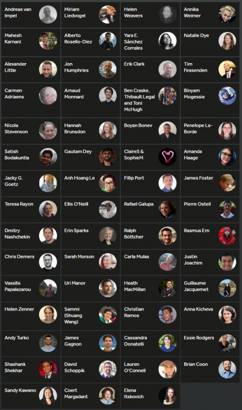
The current preLighter community
What’s in it for me?
This is a great opportunity for you to gain experience in science writing. You will get editing feedback from us and your peers and we aim to raise your profile as a trusted preprint selector and commentator. You will grow your professional network, and we are happy to support you by offering recommendation letters or in other ways.
But there is also a commitment; we expect you to select and highlight a preprint every one-or-two months.
We might not be able to accept all applicants, but are looking forward to welcoming our new preLighters.
You can find our recently published Nature paper here
Our story began two decades ago when my mentor, Klaus H. Kaestner, identified and cloned the transcription factor FOXL1, as being expressed in the mesenchyme of the mouse fetal gut (Kaestner et al. 1997). The position of FOXL1+ mesenchymal cells in such close proximity to the developing epithelium, as evidenced from In-Situ hybridization studies, suggested that FOXL1-expressing cells might be prime candidates to be key signal givers to the developing and adult gastrointestinal tract.
The early studies focused on the role of FOXL1 itself in regulating the intestinal epithelia by deriving mice homozygous for a FOXL1 null allele (FOXL1 -/-) (Perreault et al. 2001; Katz et al. 2004). FOXL1 null mice exhibit increased epithelial proliferation along with increased activation of the Wnt/β-catenin pathway, linking FOXL1 to Wnt/β-catenin pathway regulation.
The breakthrough came with a change in thinking. Klaus first realized that in order to study the role of FOXL1+ CELLS we should employ FOXL1 as a marker to trace these cells and genetically ablate them. The Kaestner lab derived two mouse models to kill FOXL1+ cells through the use of diphtheria toxin administration; FOXL1hDTR BAC transgenic mice that express the human diphtheria toxin receptor from a 170kb bacterial artificial chromosome that harbors all regulatory elements to direct transgene expression in subepithelial telocytes and Rosa-iDTR mice generated by crossing FOXL1Cre mice to a strain that produces the diphtheria toxin receptor from the ubiquitous Rosa26 locus in a Cre-dependent manner (Buch et al. 2005, Sackett et al. 2007).
Inducible ablation of FOXL1+ cells in adult mice caused a dramatic disruption to the intestinal epithelium, loss of stem and progenitor cell proliferation and the experimental mice died a few days after loss of telocytes had been initiated, demonstrating that FOXL1+ cells play a major role in stem cell function (Aoki et al. 2016).
I joined the Kaestner lab for my post-doctoral training during the time when these cell ablation models where being characterized in details. I am trained as a developmental biologist and therefore studying the potential cross talk between epithelia and mesenchyme was of great interest to me, even though at the time very little was known about the nature and function of FOXL1+ cells. In fact, we had no way to detect FOXL1 protein in tissue sections or biochemically, as multiple attempts at obtaining anti-FOXL1 antibodies by commercial outfits had been unsuccessful.
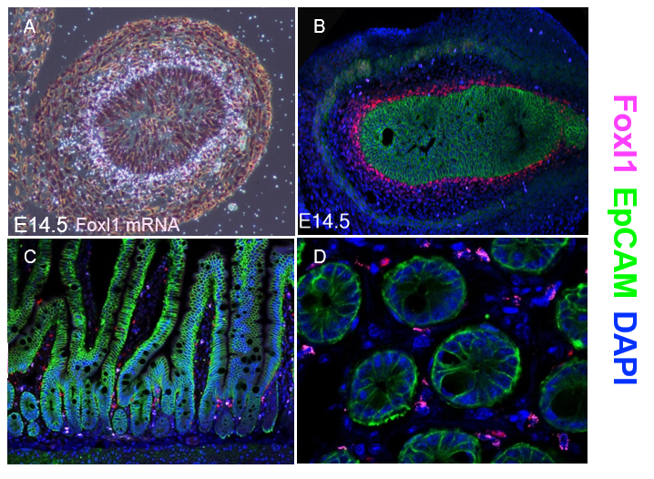
Thankfully, Chris V. E. Wright’s lab at Vanderbilt University came to our aid and generated multiple monospecific anti-FOXL1 antibodies for us. Antibody staining of mouse fetal gut showed a protein expression pattern for FOXL1 that was very similar to the one seen two decades earlier using radioactive In-situ hybridization to detect FOXL1-mRNA (Kaestner et al. 1997) (Figure 1 A-B).
However, the immunostaining for FOXL1 protein in the adult mouse intestine was disappointing at first. FOXL1 protein was present in the nuclei of selected mesenchymal cells; However, the abundance was very low (Figure 1C-D). On average, there were two to three FOXL1+ cells per crypt and their location was at mid-crypt region and along the villi core, in-addition to the crypt base where the stem cells reside.
Figure 1. FOXL1 marks a subset of mesenchymal cells during mouse development and in adult gastrointestinal tissue. (A-B) Mouse fetal gut E14.5 demonstrating by radioactive labeled probe (A) and immunofluorescence staining (B) nuclear FOXL1 mRNA (A) and protein (B) expression (red) in mesenchymal cells located in close apposition to the endoderm during development (outlined with immunofluorescence for EpCAM, green). (C-D) Sections of adult proximal jejunum, longitudinal section (C) and transverse section within the crypts region (D) showing FOXL1 expression localized to the nuclei of mesenchymal cells surrounding the crypt zone as well as alongside the villus core.
It is well known that the driving force for intestinal stem cell function is the Wnt/β-catenin pathway, which acts as a short range signaling-system. Potential cell types that might provide Wnt ligands should be in close contact with the stem cells. Do FOXL1+ cells touch stem cells? Do FOXL1+ cells express Wnts? Do they provide the essential Wnts that maintain stem cell identity? These were the key questions that I set out to answer.
With these questions in mind, I met Chris Wright for the first time in person, at the Gastrointestinal tract FASEB meeting in August 2015. During our little discussion, Chris mentioned “cytonemes”, cellular projections that are specialized for exchange of signaling molecules, and suggested that I investigate FOXL1+ cell structure. If FOXL1+ cells have long extensions and/or posses a unique cell structure, this might allow them to contact all epithelial cells.
Back in the lab, I had a clearer understanding as to which steps I should take –
I planned to inhibit all Wnt secretion from FOXL1+ cells and ask: Are stem cells affected?
I needed to sort GFP-labeled FOXL1+ cells (using a FOXL1-Cre ;Rosa-YFP mice) and prepare RNA seq libraries. Determine their gene expression profile: Do FOXL1+ express Wnts, and if so which ones?
I had to label FOXL1+ cells with a membrane reporter so that I could determine the extent of FOXL1+ cell structure
Targeting secretion of all 19 mammalial Wnt proteins can be done by deleting either Wntless or Porcupine, two essential Wnt processing enzymes, for which floxed mutant mice were already available. In order to inhibit Wnt secretion from adult and not fetal FOXL1+ cells, I need an inducible-FOXL1 driven Cre. With the help of fellow postdoc Kirk Wangensteen, I built a FOXL1-CreERT2 BAC and generated a new transgenic mouse line.
The next challenge arose when I tried to sort GFP-labeled FOXL1+ cells. To be able to sort FOXL1+ cells I had to selectively digest the mesenchyme from the intestinal epithelium in a single cell suspension. It was difficult to determine the optimal conditions to digest the mesenchyme as harsh digestion killed FOXL1+ cells, while mild digestion did not liberate any GFP-positive cells. Together with fellow postdoc Yue Wang, we devised a strategy to enable the selection to be successful. We isolated FOXL1+ cells, made RNA seq libraries and submitted them for sequencing.
The last piece of the puzzle was determinning FOXL1+ cell structure. To achieve this goal, I crossed our FOXL1 Cre mice to the Rosa-mTmG reporter in which FOXL1 promoter driven Cre activity lead to the expression of a membrane-bound version of GFP, which labeled the plasma membrane and allowed me to see the full extent of FOXL1+ cell.
The results were impressive; FOXL1+ GFP labeled cells were very large in extent and thus in contact with the entire epithelium from crypt base to the tip of the villi, with each and every single epithelial cell being touched by FOXL1+ mesenchymal cells!
During the same week I determined FOXL1+ cell structure, the RNAseq data was returned from sequencing. FOXL1+ cells indeed express a specific subset of Wnts and also the Wnt pathway inducers, R-Spondins. However, FOXL1+ cells also made high levels of Wnt inhibitors as well as BMPs, which are known to oppose Wnt signaling. How could this be, as we had shown through cell ablation that critical Wnt signals emanate from FOXL1+ cells?
I reasoned that since I had sorted FOXL1+ cells from anywhere along the crypt-villus axis for my RNAseq study, FOXL1+ cells might compartmentalize expression of signaling molecules based on their specific position along the crypt-villus axis.
To test this hypothesis, I contacted Shalev Itzkovitz from the Weizmann Institute, who had optimized a single molecule mRNA-Fluorescence In-Situ Hybridization (smFISH) technique for the mouse intestine. My goal was to focus on mRNA localization of different signaling molecules in FOXL1+ cell projections along the crypt-villus.
For this, I had to devise a way to label the full extent of FOXL1 cells, not just their nuclei. Unfortunately, I could not employ my Foxl1Cre Rosa-mTmG mice, as the reporter has a global tomato fluorescent protein expression, which bleeds through all analysis channels, thereby interfering with the smFISH signal. FOXL1 antibody staining would also not work, as it would label only the nuclei. What I needed was to identify a surface marker that could be specifically used to label the cells.
The RNAseq data revealed high expression of platelet derived growth factor receptor α (PDGFRα), member of the “villus cluster genes” characterized previously during gut development (Walton et al., 2012, Shyer et al., 2013, Shyer et al., 2015, Walton et al., 2016). Does PDGFRα label FOXL1+ cells? And if so, would it be possible to use it as a marker to label FOXL1+ cell extensions? YES! We demonstrated that all FOXL1+ cells are PDGFRα+.
In Shalev’s lab, Beáta Tóth combined PDGFRα immunostaining with smFISH and we were able to show regional differentiation in mRNA localization of different signaling molecules along FOXL1+ projections, with FOXL1+ cells near the crypt bottom producing abundant Wnt2b, a canonical Wnt pathway activator, while those further up the crypt-villus axis expressed high levels of Wnt pathway inhibitors.
I was puzzled by the unusual structure of FOXL1+ cells, which I also confirmed by electron microscopy. These cells are extremely thin but very large, with diameters in excess of 200 micrometer (for comparison, an intestinal epithelial cell is only about 10 micrometer in size). I was wondering if such unique stromal cells had been described in the literature, based on histological technologies.
Popescu named these cells “Telocytes” from the Greek words “telos” meaning end, “cytes” meaning cells. Telocytes are cells characterized by extremely long and thin projections called telopodes that may reach millimeters long and express PDGFRα in both human and mouse gut.
Apparently, neurons are not unique; telocytes also have long extensions that make direct contact with each other. Would it be possible to use the neuroscientists’ technology to study the 3D network of these cells? X-CLARITY is a method designed by neuroscientists for clearing tissues in order to visualize neurons in their 3D structure within the brain without the need for sectioning (Chung and Deisseroth 2013). Could we apply this technique to clear the intestine and visualize telocytes in their 3D structure?
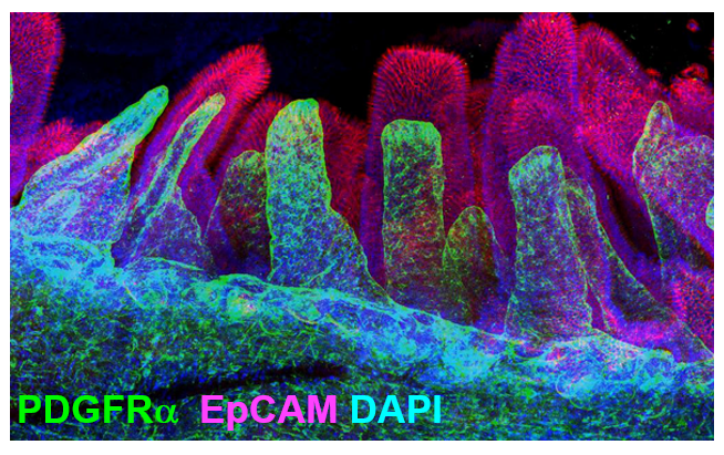
In fact, clearing whole intestine and immunostaining for PDGFRα in green and EpCAM to label epithelial cells in red, allowed me to visualize the comprehensive stromal network of telocytes that form a plexus that supports the entire epithelium (Figure 2).
Figure 2. The 3D network of subepithelial telocytes in the adult intestine. Confocal imaging of cleared mouse whole small intestine using X-CLARITY. Immunofluorescence staining for PDGFRα (green) and EpCAM (red) showing the subepithelial network of telocytes.
My journey has just begun, and many exciting questions remain: Does FOXL1 label all telocytes? What is the origin of this remarkable cell? How and when do cells acquire telocyte characteristics? How do these cells compartmentalize signaling? What are the mechanisms by which telocytes signal to the epithelium.
A postdoctoral position is available in the laboratory of Dr. Lei Lei, in the Department of Cell and Developmental Biology, University of Michigan Medical School.
The research in the Lei lab focuses on cellular and molecular mechanisms underlying mammalian oogenesis. We are particularly interested in how the primordial follicle pool (i.e. ovarian reserve) forms during fetal ovarian development and is maintained in adult ovaries. The research in the Lei lab utilize broad cellular and molecular experimental approaches, including genetic mouse models, in vitro organ culture, live-imaging, single-cell lineage tracing, RNA-sequencing and proteomics.
The Lei Lab is seeking a highly motivated postdoctoral researcher to investigate the mechanism of intercellular bridge formation during fetal germ cell development, and the role of intercellular bridges in oocyte differentiation. The goal of this project is to identify novel fetal origins of adult ovarian diseases. Candidates must have a Ph.D. in biological science. Candidates should send a cover letter describing current research interests, a CV and the names and contact information of three references to Dr. Lei Lei (leile@med.umich.edu)
The Nerurkar Lab is looking for Postdoctoral Researchers with an interest in the interplay between molecular and mechanical aspects of vertebrate morphogenesis. Using the chick embryo, we combine live in vivo imaging, embryology and molecular genetics with engineering and physics approaches to study how developmental signals modulate physical forces that shape the embryo, and how forces in turn feedback on tissue growth and stem cell differentiation. Projects include early morphogenesis and patterning of the gut tube and brain, and organogenesis of the small intestine. Applicants must hold a PhD in molecular biology, development, bioengineering, or related field. Individuals with an embryology background who are interested in building an expertise in biophysical and quantitative approaches to development are particularly encouraged to apply.
Part of the Department of Biomedical Engineering at Columbia University, the Nerurkar Lab is located on the Morningside Heights campus of Columbia University in the City of New York. An academic reflection of New York’s excitement and creativity, Columbia offers a rich research environment, with boundless opportunities for collaboration with experts across engineering, biology, and clinical/translational disciplines. Interested applicants should contact Nandan Nerurkar at nln2113@columbia.edu.
Looking to conduct research in molecular biology and genetics? We are looking for a lab technician to assist in research on muscle stem cells, development, regeneration, disease, and evolution. More details about our research can be found at http://www.kardonlab.org/. Technician will assist in management of a mouse colony as well as conduct supervised research (leading to publications). Technician must be reliable, well organized, detail-oriented, excited about research and committed to working in our lab for at least two years. Prior lab experience is preferred (although not necessarily required), and class work in biology and enthusiasm for science is essential. Lab is located at the University of Utah in Salt Lake City, affording amazing opportunities for science and outdoor recreation. Looking for someone to start June-July 2018.
Please contact Gabrielle Kardon (gkardon@genetics.utah.edu) with CV, list of references, and a brief statement about why you are interested in the position. BS or BA required.
the GOEvol consortium proudly presents its 6th meeting #Sensation @GOEEvolution 2018 taking place in Göttingen from September 27th to 28th 2018.
The perception of environmental stimuli, their processing and integration is essential for any organism. Apart from the more familiar senses like hearing, seeing or tasting, there are sensory tasks performed by highly specialized animals, such as echolocation in bats or the perception of polarized light in insects. Sensory processing consequently also differs strongly between species. However, at the same time there are astonishing similarities between sensory modalities of phylogenetically distant animal groups, such as the shared cellular structure of light-sensitive organs or the genetic control and developmental origin of sensory cells. With methodological innovation, more and more species can be used for detailed analyses, which further expand the understanding of the evolution of sensation.
Because of the diversity of research and various methodologies in multiple (emerging) model organisms in the field of evolution of sensation we want to bring together scientists from a broad range of fields to reveal commonalities across disciplines.
Following the GOEvol tradition, we aim for an interdisciplinary symposium with an informal atmosphere with plenty of possibilities for social networking. If you enjoy small interactive meetings and the topic suits you, come along!
There are several slots for contributing talks and poster presentations. We strongly encourage interested students and researchers from all levels (Bachelor, Master, PhD and above) to register and apply for talks and poster presentations.
Moreover, we want to support parents to participate. Therefore, depending on the demand, we will be able to provide childcare as well as designated rooms for nursing.
Costs to register are 10€ for students, 20€ for Postdocs and PIs.
Invited speakers:
Sally Leys (University of Alberta, Canada)
Michael Bok (University of Bristol, UK)
Tobias Kaiser (MPI for Evolutionary Biology, Plön, Germany)
Robert Barton (University of Durham, UK)
Mirjam Knörnschild (Free University of Berlin, Germany)
Brigitte Schoenemann (University of Cologne, Germany)


 (No Ratings Yet)
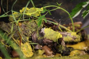
 (1 votes)
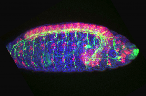


 Costs to register are 10€ for students, 20€ for Postdocs and PIs.