A postdoctoral research position is available in the laboratory of Dr. Kristin Gribble at the Marine Biological Laboratory, Woods Hole, MA. The interests of the lab include the mechanisms and evolution of the biology of aging, and maternal and transgenerational effects on offspring health. We use rotifers as a model system for our work. For more information about our lab’s work and a list of publications, see mbl.edu/jbpc/gribble.
Qualified applicants will have the opportunity to study the genetic and epigenetic mechanisms of aging in a novel experimental model system, focusing on how maternal effects influence offspring health and lifespan. This NSF-CAREER funded research program will use experimental, genetic, biochemical, and bioinformatic approaches to elucidate the mechanisms of transgenerational epigenetic inheritance.
Applicants should posses a Ph.D. in molecular biology, cell biology, biochemistry, genetics, bioinformatics, or a related field. The ideal candidate will have a record of scientific rigor, productivity, and creativity; the ability to work independently and as part of a team; and a strong publication record. Excellent oral and written communication skills are required. Highly motivated individuals with experience in other model systems and a background in biochemistry, cell/molecular biology, epigenetics, and/or bioinformatics are encouraged to apply. Salary will be commensurate with experience and qualifications.
Applicants must apply for this position via the Marine Biological Laboratory careers website. Please submit: a cover letter with a brief description of your research experience and how your expertise will contribute to research on the mechanisms of parental effects and transgenerational inheritance; a CV including a list of publications, and contact information for three references.
The new Center for Stem Cell & Organoid Medicine (CuSTOM) at Cincinnati Children’s Hospital Medical Center (CCHMC) is launching a major new initiative to recruit outstanding tenure-track or tenured faculty at the Assistant to Associate Professor level.
CuSTOM (www.cincinnatichildrens.org/custom) is a multi-disciplinary center of excellence integrating developmental and stem cell biologists, clinicians, bioengineers and entrepreneurs with the common goal of accelerating discovery and facilitating bench-to-bedside translation of organoid technology and regenerative medicine. Faculty in CuSTOM benefit from the unique environment and resources to studies of human development, disease and regenerative medicine using pluripotent stem cell and organoid platforms.
CCHMC is a leader in organoid biology and one of the top ranked pediatric research centers in the world, providing a unique environment for basic and translational research. Among pediatric institutions CCHMC is the third-highest ranking recipient of research grants from the National Institutes of Health. CCHMC continues to make major investments in research supporting discovery with 1.4 million square feet of research space and subsidized state-of-the-art core facilities including a human pluripotent stem cell facility, CRISPR genome editing, high-throughput DNA analysis, biomedical informatics, a Nikon Center of Excellence imaging core and much more.
We invite applications from innovative and collaborative investigators focused on basic or translational research in human development and/or disease using stem cells or organoid models. Successful candidates must hold the PhD, MD, or MD/PhD degrees, and will have a vibrant research program with an outstanding publication record.
Applicants should submit their curriculum vitae, two to three page research statement focused on future plans, and contact information for three people who will provide letters of recommendation to CuSTOM@cchmc.org. Applications must be submitted by December 1st, 2020
The Cincinnati Children’s Hospital Medical Center, and the University of Cincinnati are Affirmative Action/Equal Opportunity Employers, fostering diversity and inclusion. Qualified women and minority candidates are especially encouraged to apply.
In the latest episode of Genetics Unzipped, Kat Arney looks at the ancient war between our genes and the pathogens that infect us, going back thousands of years to the Black Death and before, through to our very latest foe: the SARS-CoV-2 coronavirus behind COVID-19.
With Claire Steves (King’s College London), Christiana Scheib (University of Tartu) and Lucy van Dorp (UCL).
If you enjoy the show, please do rate and review on Apple podcasts and help to spread the word on social media. And you can always send feedback and suggestions for future episodes and guests to podcast@geneticsunzipped.com Follow us on Twitter – @geneticsunzip
The neocortex is the seat of our higher cognitive abilities that distinguish us from other mammals and that make us human (Rakic, 2009). One basis for this crucial feature is the increase in the size of the neocortex during hominin evolution, culminating in modern humans (Striedter, 2005, Azevedo et al., 2009, Kaas, 2013, Sousa et al., 2017, Molnar et al., 2019). A key issue in this context is the identification of genomic determinants that underlie the increased growth of the neocortex during brain development. Once candidate genes have been identified, the challenge then is to demonstrate their role in neocortex expansion in an appropriate system. Here, we summarize the background information that suggested the human-specific gene ARHGAP11B to be a candidate to have contributed to neocortex expansion and folding during human evolution, and explain the rationale for demonstrating this role in an ARHGAP11B-transgenic non-human primate model system, that is, fetuses of the common marmoset. Such functional, developmental and evolutionary studies have so far been rarely performed in transgenic non-human primates. In our recent publication, Heide et al. 2020, we show that the human-specific gene ARHGAP11B, when expressed to physiological levels in the fetal marmoset neocortex, indeed causes neocortex expansion and increases neocortex folding, implying that this gene significantly contributed to human neocortex evolution (Heide et al., 2020). Moreover, we hope that our findings provide evidence in support of the usefulness and feasibility of genetically modified non-human primates for neurodevelopmental and evolutionary studies, as well as other fields of neurobiology.
A need for genetically modifiable non-human primate models in neurobiological studies
Which systems are most appropriate for studying the development of the neocortex with the aim to gain insight into the development and evolution of the human neocortex? Commonly used animal models that lend themselves to genetic modifications have been smooth-brained (lissencephalic) rodents (mouse, rat) and the ferret, a carnivore with a folded (gyrencephalic) brain (Molnar et al., 2006, Sun and Hevner, 2014, Kawasaki, 2018, Zhao and Bhattacharyya, 2018). However, many findings about neocortical development obtained in these model systems cannot be translated as such to humans, as is exemplified, in particular, in the case of many mouse disease models (e.g., mouse models of primary microcephaly (Pinson et al., 2019)).
A recently emerged, promising in vitro model system of human neocortical development that overcomes some of these limitations are human brain organoids (Kadoshima et al., 2013, Lancaster et al., 2013, Camp et al., 2015, Qian et al., 2016, Quadrato et al., 2017). These are 3D cellular assemblies that model the tissue of certain brain regions over a particular developmental time window and recapitulate many aspects of the cytoarchitecture and cell-type complexity of the modelled brain tissue (Heide et al., 2018). Moreover, comparison of brain organoids of human vs. non-human primate origin (macaque, chimpanzee, orang-utan) has led to the identification of human-specific features of neocortical development (Otani et al., 2016, Mora-Bermudez et al., 2016, Pollen et al., 2019, Kanton et al., 2019). Importantly, brain organoids can easily be genetically modified (Fischer et al., 2019), and human brain organoids have been shown to recapitulate gene expression patterns of fetal human neocortex (Camp et al., 2015). However, despite its promise, the brain organoid model system still has certain limitations, such that is does not fully recapitulate the cytoarchitecture, cell-type composition and late and postnatal stages of neocortex development (Heide et al., 2018). Moreover, cell-type specification in brain organoids seems to be impaired due to cellular stress (Bhaduri et al., 2020).
Hence, fetal human brain tissue ex vivo (Rakic, 2006, Florio et al., 2015, Johnson et al., 2015, Pollen et al., 2015, Kalebic et al., 2019, Namba et al., 2020) and non-human primate models (Smart et al., 2002, Rakic, 2006, Kelava et al., 2012, Garcia-Moreno et al., 2012, Betizeau et al., 2013) have been increasingly used to overcome the limitations of the rodent and ferret models and of brain organoids for studying the development of the neocortex with the aim to gain insight into the development and evolution of the human neocortex. However, the use of fetal human brain tissue ex vivo is limited to early stages of neocortical development, and genetic modification approaches can only be conducted – for obvious ethical reasons – with ex vivo fetal human brain tissue. It is for these reasons that genetically modifiable non-human primate models have recently emerged as system of choice to gain insight into human neocortex development and evolution (Sasaki et al., 2009, Niu et al., 2010, Niu et al., 2014, Shi et al., 2019, Heide et al., 2020). A major advantage of non-human primate models is that in terms of morphology, cell-type composition, gene expression and interaction partners, these models are much closer to human neocortex development than the rodent and ferret models. Moreover, genetically modifiable non-human primate models are likely to have huge potential in generating models of neurological and neurodevelopmental disorders.
ARHGAP11B — a human-specific gene that may drive human neocortex expansion and folding?
The ARHGAP11B gene evolved ~5 mya, that is, after the split of the lineage leading to modern humans and the lineage leading to chimpanzee and bonobo, by segmental duplication of the widespread gene ARHGAP11A (Sudmant et al., 2010). In other words, ARHGAP11B is only found in humans and hence is a human-specific gene. However, ARHGAP11B is not a simple copy of ARHGAP11A, as the ARHGAP11B protein corresponds to only the N-terminal one quarter of the ARHGAP11A protein and, importantly, possesses a unique, human-specific 47 amino acid sequence in its C-terminal domain that is key for its function (Florio et al., 2015, Namba et al., 2020). This unique C-terminal protein sequence arises from a single C-to-G nucleotide substitution in ARHGAP11B that generated a novel splice donor site, resulting in the loss of 55 nucleotides upon mRNA splicing. This loss in turn causes a shift in the reading frame, leading to ARHGAP11B’s unique C-terminal 47 amino acid sequence (Florio et al., 2016). Previous functional analyses by strong overexpression of this gene in embryonic mouse (Florio et al., 2015) and ferret (Kalebic et al., 2018) neocortex showed increased numbers of basal progenitor cells and of upper-layer neurons, the class of progenitors and type of cortical neurons, respectively, that have been implicated in neocortex expansion (Lui et al., 2011, Fame et al., 2011, Borrell and Reillo, 2012, Betizeau et al., 2013, Florio and Huttner, 2014, Dehay et al., 2015, Lodato and Arlotta, 2015). Moreover, in the case of mouse, ARHGAP11B overexpression could induce folding of the normally smooth neocortex (Florio et al., 2015). These findings suggested that ARHGAP11B is a candidate gene to have contributed to neocortex expansion and folding during human evolution. However, the key question was whether this gene, when expressed to physiological levels and in a primate model that is evolutionarily closer to human than mouse or ferret, would increase neocortex size and folding.
Which genetically modifiable non-human primate model to choose?
We therefore searched for a genetically modifiable primate model that is evolutionarily as close as (ethically) possible to human and that possesses all relevant stem cell populations at the correct relative abundance in the developing neocortex, to allow us to explore the potential role of ARHGAP11B in the expansion of the neocortex during development and human evolution. This confined our choice to two non-human primate models, the common marmoset (Callithrix jacchus) and the macaque (eitherMacaca mulatta or Macaca fascicularis). We chose to focus on the marmoset, as this New World monkey, while exhibiting many of the features of the large and folded human neocortex, has – in contrast to the macaque – a small and unfolded neocortex, making it thus an ideal model to study ARHGAP11B’s potential contribution to neocortical expansion and folding.
ARHGAP11B increases fetal primate neocortex size and folding
In Heide et al. 2020, we generated, in collaboration with the research groups of Erika Sasaki and Hideyuki Okano in Japan who have pioneered the transgenic marmoset technology (Sasaki et al., 2009), ARHGAP11B-transgenic marmoset fetuses (Figure A) that expressed ARHGAP11B in the developing neocortex under the control of its own, human promoter (Heide et al., 2020).
(A) Cartoon depicting the timeline of the generation of ARHGAP11B-transgenic fetal marmosets. (B) Schematic showing a section through the neocortical wall (left) and brain images (right) of wildtype (WT) and ARHGAP11B-transgenic marmoset fetuses at 101 days of pregnancy; arrowheads, folds; orange dashed line, rostral boundary of wildtype (WT) and ARHGAP11B-transgenic fetal marmoset neocortex; yellow dashed line, caudal boundary of wildtype (WT) fetal marmoset neocortex; red dashed line, caudal boundary of ARHGAP11B-transgenic fetal marmoset neocortex; scale bars, 1 mm.
In the neocortex of these ARHGAP11B-transgenic marmoset fetuses, ARHGAP11B was expressed to physiological levels, that is, to similar levels as in fetal human neocortex, and its expression within the neocortex was confined to neural stem and progenitor cells (Heide et al., 2020). Furthermore, this ARHGAP11B expression increased the abundance of basal radial glia (Heide et al., 2020) – the basal progenitor cell type thought to play a key role in neocortex expansion and folding, notably in human neocortex development (Lui et al., 2011, Borrell and Reillo, 2012 Florio and Huttner, 2014). This was accompanied by an increase in upper-layer neurons (Heide et al., 2020) — the cortical neuron type thought to strongly contribute to our higher cognitive abilities (Fame et al., 2011). At the supracellular level, this ARHGAP11B expression resulted in increased neocortex size and induced folding of the normally unfolded fetal marmoset neocortex (Heide et al., 2020) (Figure B). In summary, our study strongly suggests that ARHGAP11B did contribute to neocortex expansion and folding in the course of human evolution.
Ethical considerations
Experiments involving non-human primates have been under constant public and scientific debate, and it is perfectly legitimate to scrutinize whether or not such experiments are really necessary and to ask whether other animal model systems are available that are appropriate to address the same scientific questions. Furthermore, experiments involving non-human primates should be performed according to the highest ethical standards.
In our case, we reasoned that in order to answer the question whether the human-specific gene ARHGAP11B contributed to neocortex expansion and folding during human evolution, it was necessary to express ARHGAP11B in a suitable non-human primate model, that is, the common marmoset. We limited these experiments and analyses to fetal stages, for two main reasons. First, should ARHGAP11Bexpression increase neocortex size and neuron numbers as we anticipated, the consequences for the postnatal and adult marmosets with regard to behaviour and nervous system performance might be unpredictable. In this context, one should realize that increases in neocortex size and neuron numbers are not necessarily beneficial but can be the underlying cause of certain human diseases (e.g., megalencephaly, polymicrogyria), and accordingly could lead to suffering of the animals (e.g., from seizures). To avoid generating ARHGAP11B-expressing postnatal and adult marmosets, all ARHGAP11B-expressing marmoset fetuses analyzed in our study were newly and individually generated (rather than being descendants of an ARHGAP11B-expressing marmoset line). Second, our previous data had indicated that ARHGAP11B expression increased basal progenitors and upper-layer neurons during the development of the neocortex. This suggested that in our case an analysis of fetal stages of ARHGAP11B-expressing marmosets would be appropriate and constructive, and would allow closely monitoring neocortex development and analyzing it at the relevant stages.
We hope that our study shows that genetically modified non-human primate fetuses can be superior models to understand human neocortex development and evolution. Furthermore, our work will hopefully encourage other researchers from the present and other fields of neurobiology (including disease modelling) to study genetically modified non-human primate models in the future, as (i) such experiments can be performed in an ethically justifiable way (see above), (ii) the results may answer questions that other, non-primate models cannot answer, and (iii) the results most likely can be directly translated to humans.
References
AZEVEDO, F. A. C., CARVALHO, L. R. B., GRINBERG, L. T., FARFEL, J. M., FERRETTI, R. E. L., LEITE, R. E. P., JACOB, W., LENT, R. & HERCULANO-HOUZEL, S. 2009. Equal numbers of neuronal and nonneuronal cells make the human brain an isometrically scaled-up primate brain. J. Comp. Neurol. , 513, 532-541.
BETIZEAU, M., CORTAY, V., PATTI, D., PFISTER, S., GAUTIER, E., BELLEMIN-MÉNARD, A., AFANASSIEFF, M., HUISSOUD, C., DOUGLAS, R. J., KENNEDY, H. & DEHAY, C. 2013. Precursor diversity and complexity of lineage relationships in the outer subventricular zone of the primate. Neuron, 80, 442-457.
BHADURI, A., ANDREWS, M. G., MANCIA LEON, W., JUNG, D., SHIN, D., ALLEN, D., JUNG, D., SCHMUNK, G., HAEUSSLER, M., SALMA, J., POLLEN, A. A., NOWAKOWSKI, T. J. & KRIEGSTEIN, A. R. 2020. Cell stress in cortical organoids impairs molecular subtype specification. Nature, 578, 142-148.
BORRELL, V. & REILLO, I. 2012. Emerging roles of neural stem cells in cerebral cortex development and evolution. Dev Neurobiol, 72, 955-971.
CAMP, J. G., BADSHA, F., FLORIO, M., KANTON, S., GERBER, T., WILSCH-BRÄUNINGER, M., LEWITUS, E., SYKES, A., HEVERS, W., LANCASTER, M., KNOBLICH, J. A., LACHMANN, R., PÄÄBO, S., HUTTNER, W. B. & TREUTLEIN, B. 2015. Human cerebral organoids recapitulate gene expression programs of fetal neocortex development. Proc Natl Acad Sci U S A, 112,15672-7.
DEHAY, C., KENNEDY, H. & KOSIK, K. S. 2015. The outer subventricular zone and primate-specific cortical complexification. Neuron, 85, 683-694.
FAME, R. M., MACDONALD, J. L. & MACKLIS, J. D. 2011. Development, specification, and diversity of callosal projection neurons. Trends Neurosci, 34, 41-50.
FISCHER, J., HEIDE, M. & HUTTNER, W. B. 2019. Genetic modification of brain organoids. Front Cell Neurosci, 13, 558.
FLORIO, M., ALBERT, M., TAVERNA, E., NAMBA, T., BRANDL, H., LEWITUS, E., HAFFNER, C., SYKES, A., WONG, F. K., PETERS, J., GUHR, E., KLEMROTH, S., PRUFER, K., KELSO, J., NAUMANN, R., NÜSSLEIN, I., DAHL, A., LACHMANN, R., PÄÄBO, S. & HUTTNER, W. B. 2015. Human-specific gene ARHGAP11B promotes basal progenitor amplification and neocortex expansion. Science, 347, 1465-1470.
FLORIO, M. & HUTTNER, W. B. 2014. Neural progenitors, neurogenesis and the evolution of the neocortex. Development, 141, 2182-2194.
FLORIO, M., NAMBA, T., PÄÄBO, S., HILLER, M. & HUTTNER, W. B. 2016. A single splice site mutation in human-specific ARHGAP11B causes basal progenitor amplification. Sci Adv, 2,e1601941.
GARCIA-MORENO, F., VASISTHA, N. A., TREVIA, N., BOURNE, J. A. & MOLNAR, Z. 2012. Compartmentalization of cerebral cortical germinal zones in a lissencephalic primate and gyrencephalic rodent. Cereb. Cortex, 22, 482-492.
HEIDE, M., HAFFNER, C., MURAYAMA, A., KUROTAKI, Y., SHINOHARA, H., OKANO, H., SASAKI, E. & HUTTNER, W. B. 2020. Human-specific ARHGAP11B increases size and folding of primate neocortex in the fetal marmoset. Science, eabb2401 [published online ahead of print].
HEIDE, M., HUTTNER, W. B. & MORA-BERMUDEZ, F. 2018. Brain organoids as models to study human neocortex development and evolution. Curr Opin Cell Biol, 55, 8-16.
JOHNSON, M. B., WANG, P. P., ATABAY, K. D., MURPHY, E. A., DOAN, R. N., HECHT, J. L. & WALSH, C. A. 2015. Single-cell analysis reveals transcriptional heterogeneity of neural progenitors in human cortex. Nat. Neurosci., 18, 637-646.
KAAS, J. H. 2013. The evolution of brains from early mammals to humans. WIREs Cogn. Sci., 4, 33-45.
KADOSHIMA, T., SAKAGUCHI, H., NAKANO, T., SOEN, M., ANDO, S., EIRAKU, M. & SASAI, Y. 2013. Self-organization of axial polarity, inside-out layer pattern, and species-specific progenitor dynamics in human ES cell-derived neocortex. Proc Natl Acad Sci U S A, 110, 20284-9.
KALEBIC, N., GILARDI, C., ALBERT, M., NAMBA, T., LONG, K. R., KOSTIC, M., LANGEN, B. & HUTTNER, W. B. 2018. Human-specific ARHGAP11B induces hallmarks of neocortical expansion in developing ferret neocortex. eLife, 7, e41241.
KALEBIC, N., GILARDI, C., STEPIEN, B., WILSCH-BRÄUNINGER, M., LONG, K. R., NAMBA, T., FLORIO, M., LANGEN, B., LOMBARDOT, B., SHEVCHENKO, A., KILIMANN, M. W., KAWASAKI, H., WIMBERGER, P. & HUTTNER, W. B. 2019. Neocortical expansion due to increased proliferation of basal progenitors is linked to changes in their morphology. Cell Stem Cell, 24, 535-550 e9.
KANTON, S., BOYLE, M. J., HE, Z. S., SANTEL, M., WEIGERT, A., SANCHIS-CALLEJA, F., GUIJARRO, P., SIDOW, L., FLECK, J. S., HAN, D. D., QIAN, Z. Z., HEIDE, M., HUTTNER, W. B., KHAITOVICH, P., PÄÄBO, S., TREUTLEIN, B. & CAMP, J. G. 2019. Organoid single-cell genomic atlas uncovers human-specific features of brain development. Nature, 574, 418-422.
KAWASAKI, H. 2018. Molecular investigations of the development and diseases of cerebral cortex folding using gyrencephalic mammal ferrets. Biol Pharm Bull, 41, 1324-1329.
KELAVA, I., REILLO, I., MURAYAMA, A. Y., KALINKA, A. T., STENZEL, D., TOMANCAK, P., MATSUZAKI, F., LEBRAND, C., SASAKI, E., SCHWAMBORN, J. C., OKANO, H., HUTTNER, W. B. & BORRELL, V. 2012. Abundant occurrence of basal radial glia in the subventricular zone of embryonic neocortex of a lissencephalic primate, the common marmoset Callithrix jacchus. Cereb. Cortex, 22, 469-481.
LANCASTER, M. A., RENNER, M., MARTIN, C. A., WENZEL, D., BICKNELL, L. S., HURLES, M. E., HOMFRAY, T., PENNINGER, J. M., JACKSON, A. P. & KNOBLICH, J. A. 2013. Cerebral organoids model human brain development and microcephaly. Nature, 501, 373-9.
LODATO, S. & ARLOTTA, P. 2015. Generating neuronal diversity in the mammalian cerebral cortex. Annu. Rev. Cell Dev. Biol., 31, 699-720.
LUI, J. H., HANSEN, D. V. & KRIEGSTEIN, A. R. 2011. Development and evolution of the human neocortex. Cell, 146, 18-36.
MOLNAR, Z., CLOWRY, G. J., SESTAN, N., ALZU’BI, A., BAKKEN, T., HEVNER, R. F., HUPPI, P. S., KOSTOVIC, I., RAKIC, P., ANTON, E. S., EDWARDS, D., GARCEZ, P., HOERDER-SUABEDISSEN, A. & KRIEGSTEIN, A. 2019. New insights into the development of the human cerebral cortex. J Anat, 235, 432-451.
MOLNAR, Z., METIN, C., STOYKOVA, A., TARABYKIN, V., PRICE, D. J., FRANCIS, F., MEYER, G., DEHAY, C. & KENNEDY, H. 2006. Comparative aspects of cerebral cortical development. Eur J Neurosci, 23, 921-34.
MORA-BERMUDEZ, F., BADSHA, F., KANTON, S., CAMP, J. G., VERNOT, B., KOHLER, K., VOIGT, B., OKITA, K., MARICIC, T., HE, Z., LACHMANN, R., PÄÄBO, S., TREUTLEIN, B. & HUTTNER, W. B. 2016. Differences and similarities between human and chimpanzee neural progenitors during cerebral cortex development. eLife, 5, e18683.
NAMBA, T., DOCZI, J., PINSON, A., XING, L., KALEBIC, N., WILSCH-BRÄUNINGER, M., LONG, K. R., VAID, S., LAUER, J., BOGDANOVA, A., BORGONOVO, B., SHEVCHENKO, A., KELLER, P., DRECHSEL, D., KURZCHALIA, T., WIMBERGER, P., CHINOPOULOS, C. & HUTTNER, W. B. 2020. Human-specific ARHGAP11B acts in mitochondria to expand neocortical progenitors by glutaminolysis. Neuron, 105, 867-881 e9.
NIU, Y., YU, Y., BERNAT, A., YANG, S., HE, X., GUO, X., CHEN, D., CHEN, Y., JI, S., SI, W., LV, Y., TAN, T., WEI, Q., WANG, H., SHI, L., GUAN, J., ZHU, X., AFANASSIEFF, M., SAVATIER, P., ZHANG, K., ZHOU, Q. & JI, W. 2010. Transgenic rhesus monkeys produced by gene transfer into early-cleavage-stage embryos using a simian immunodeficiency virus-based vector. Proc Natl Acad Sci U S A, 107, 17663-7.
NIU, Y. Y., SHEN, B., CUI, Y. Q., CHEN, Y. C., WANG, J. Y., WANG, L., KANG, Y., ZHAO, X. Y., SI, W., LI, W., XIANG, A. P., ZHOU, J. K., GUO, X. J., BI, Y., SI, C. Y., HU, B., DONG, G. Y., WANG, H., ZHOU, Z. M., LI, T. Q., TAN, T., PU, X. Q., WANG, F., JI, S. H., ZHOU, Q., HUANG, X. X., JI, W. Z. & SHA, J. H. 2014. Generation of gene-modified cynomolgus monkey via Cas9/RNA-mediated gene targeting in one-cell embryos. Cell, 156, 836-843.
OTANI, T., MARCHETTO, M. C., GAGE, F. H., SIMONS, B. D. & LIVESEY, F. J. 2016. 2D and 3D stem cell models of primate cortical development identify species-specific differences in progenitor behavior contributing to brain size. Cell Stem Cell, 18, 467-80.
PINSON, A., NAMBA, T. & HUTTNER, W. B. 2019. Malformations of human neocortex in development – their progenitor cell basis and experimental model systems. Front Cell Neurosci, 13, 305.
POLLEN, A. A., BHADURI, A., ANDREWS, M. G., NOWAKOWSKI, T. J., MEYERSON, O. S., MOSTAJO-RADJI, M. A., DI LULLO, E., ALVARADO, B., BEDOLLI, M., DOUGHERTY, M. L., FIDDES, I. T., KRONENBERG, Z. N., SHUGA, J., LEYRAT, A. A., WEST, J. A., BERSHTEYN, M., LOWE, C. B., PAVLOVIC, B. J., SALAMA, S. R., HAUSSLER, D., EICHLER, E. E. & KRIEGSTEIN, A. R. 2019. Establishing cerebral organoids as models of human-specific brain evolution. Cell, 176, 743-756.
POLLEN, A. A., NOWAKOWSKI, T. J., CHEN, J., RETALLACK, H., SANDOVAL-ESPINOSA, C., NICHOLAS, C. R., SHUGA, J., LIU, S. J., OLDHAM, M. C., DIAZ, A., LIM, D. A., LEYRAT, A. A., WEST, J. A. & KRIEGSTEIN, A. R. 2015. Molecular identity of human outer radial glia during cortical development. Cell, 163, 55-67.
QIAN, X., NGUYEN, H. N., SONG, M. M., HADIONO, C., OGDEN, S. C., HAMMACK, C., YAO, B., HAMERSKY, G. R., JACOB, F., ZHONG, C., YOON, K. J., JEANG, W., LIN, L., LI, Y., THAKOR, J., BERG, D. A., ZHANG, C., KANG, E., CHICKERING, M., NAUEN, D., HO, C. Y., WEN, Z., CHRISTIAN, K. M., SHI, P. Y., MAHER, B. J., WU, H., JIN, P., TANG, H., SONG, H. & MING, G. L. 2016. Brain-region-specific organoids using mini-bioreactors for modeling ZIKV exposure. Cell,165, 1238-1254.
QUADRATO, G., NGUYEN, T., MACOSKO, E. Z., SHERWOOD, J. L., MIN YANG, S., BERGER, D. R., MARIA, N., SCHOLVIN, J., GOLDMAN, M., KINNEY, J. P., BOYDEN, E. S., LICHTMAN, J. W., WILLIAMS, Z. M., MCCARROLL, S. A. & ARLOTTA, P. 2017. Cell diversity and network dynamics in photosensitive human brain organoids. Nature, 545, 48-53.
RAKIC, P. 2006. A century of progress in corticoneurogenesis: from silver impregnation to genetic engineering. Cereb Cortex, 16 Suppl 1, i3-17.
RAKIC, P. 2009. Evolution of the neocortex: a perspective from developmental biology. Nat. Rev. Neurosci., 10, 724-735.
SASAKI, E., SUEMIZU, H., SHIMADA, A., HANAZAWA, K., OIWA, R., KAMIOKA, M., TOMIOKA, I., SOTOMARU, Y., HIRAKAWA, R., ETO, T., SHIOZAWA, S., MAEDA, T., ITO, M., ITO, R., KITO, C., YAGIHASHI, C., KAWAI, K., MIYOSHI, H., TANIOKA, Y., TAMAOKI, N., HABU, S., OKANO, H. & NOMURA, T. 2009. Generation of transgenic non-human primates with germline transmission. Nature, 459, 523-7.
SHI, L., LUO, X., JIANG, J., CHEN, Y., LIU, C., HU, T., LI, M., LIN, Q., LI, Y., HUANG, J., WANG, H., NIU, Y., SHI, Y., STYNER, M., WANG, J., LU, Y., SUN, X., YU, H., JI, W. & SU, B. 2019. Transgenic rhesus monkeys carrying the human MCPH1 gene copies show human-like neoteny of brain development. National Science Review, 6, 480-493.
SMART, I. H., DEHAY, C., GIROUD, P., BERLAND, M. & KENNEDY, H. 2002. Unique morphological features of the proliferative zones and postmitotic compartments of the neural epithelium giving rise to striate and extrastriate cortex in the monkey. Cereb. Cortex, 12, 37-53.
SOUSA, A. M. M., MEYER, K. A., SANTPERE, G., GULDEN, F. O. & SESTAN, N. 2017. Evolution of the human nervous system function, structure, and development. Cell, 170, 226-247.
STRIEDTER, G. F. 2005. Principles of Brain Evolution, Sinauer Associates Inc.
SUDMANT, P. H., KITZMAN, J. O., ANTONACCI, F., ALKAN, C., MALIG, M., TSALENKO, A., SAMPAS, N., BRUHN, L., SHENDURE, J. & EICHLER, E. E. 2010. Diversity of human copy number variation and multicopy genes. Science, 330, 641-646.
SUN, T. & HEVNER, R. F. 2014. Growth and folding of the mammalian cerebral cortex: from molecules to malformations. Nat. Rev. Neurosci., 15, 217-232.
ZHAO, X. & BHATTACHARYYA, A. 2018. Human models are needed for studying human neurodevelopmental disorders. Am J Hum Genet, 103, 829-857.
Flowering plants, from giant sequoias to miniscule duckweed, all depend on the action of small populations of cells, called meristems, to grow. Meristems contain stem cells that continue to proliferate to give rise to roots, shoots, leaves, and branches. However, there are situations in which meristematic cells cease their proliferative activity and terminally differentiate; this occurs in flowers, and floral specific gene networks have been identified that terminate stem cell activity as flower development ensues. A far less well studied example of meristem termination is the formation of thorns. A number of plant species equip themselves with thorns to deter herbivores yet little is known of how these weapons are made.
Over ten years ago, our group set out to understand how meristematic activity is arrested during thorn development. Citrus was selected as a model for thorn development for two reasons: agronomic importance and feasibility. Citrus is one of the most economically valuable fruit crops in the world, and thornlessness is a breeding target as thorns affect fruit harvesting efficiency and can physically damage fruits. In addition, research in citrus is practical: the genome sequences of several citrus species are available, there are naturally occurring citrus variants that lack thorns, and citrus is amenable to genetic transformation. As tractable mutants are key for functional genetics studies, we established a fast and efficient citrus genome editing system by using the YAO promoter to drive Cas9 expression and employed heat stress treatments to further increase CRISPR-mediated gene editing efficiency. This system has proven to be very effective and we can now inactivate up to six genes simultaneously in primary citrus transformants in just a few months.
In our recent paper, Zhang et al 2020, we first characterized thorn growth and defined stages from primordium initiation to terminal differentiation. At early stages, the thorn primordia appear dome-shaped, like that of typical shoot meristems. By stage 7, the thorn tip narrows and at stage 8, thorns elongate and become pointed. Furthermore, the expression of two meristem-expressed genes, SHOOT MERISTEMLESS (STM) and WUSCHEL (WUS) are downregulated at stage 8, with STM expression becoming confined to vascular tissues and WUS expression becoming undetectable. Cell division completely ceases by stage 13, and the thorn lignifies to produce the sharp hard stiletto-like tip.
The question that naturally arises is what terminates thorn meristem gene expression at stage 8. Using a thornless Mexican lime natural variant in comparison to normal Mexican limes, we performed transcriptome analyses of young shoots. We focused on differentially expressed transcription factors that are expressed preferentially in young thorns. One candidate gene, THORN IDENTITY1, encodes a TCP transcription factor, and its homologues control bud dormancy in other plant species and so was an excellent candidate for further analyses. Interestingly, TI1 expression starts at stage 8, and a CRISPR-induced mutation of TI1 leads to the transformation of some thorns into branches. TI1 has a paralogue in citrus, TI2, whose expression in thorns starts from stage 7, and a ti2 mutation also shows the thorn transformed into branch phenotype. Mutation of TI1 and TI2 together transforms nearly every thorn into a branch, resulting in a very bushy phenotype (Figure 1).
Figure 1 Mutation of THORN IDENTITY genes converts thorns into branches. Left, control plant; right, ti1 ti2 double mutant. From Zhang et al, Current Biology, 2020: doi: 10.1016/j.cub.2020.05.068.
WUS expression is upregulated in ti1, ti2 and ti1ti2 mutants, suggesting that the TI genes may function through repressing WUS transcription. Supporting this, both TI1 and TI2 repress WUS promoter activity in transient expression assays, and TI1 directly binds to the WUS promoter as demonstrated by both chromatin immunoprecipitation and gel shift assays. Interestingly, the citrus WUS promoter has a TCP consensus binding site that is not present in the model plant Arabidopsis thaliana, and we showed that mutation of this cis-element can abolish TI1-WUS promoter regulation. Finally, disruption of the TI1–WUS pathway by either ectopic expression of WUS or via a WUS promoter mutation affects thorn development, indicating that this pathway is critical for thorn growth.
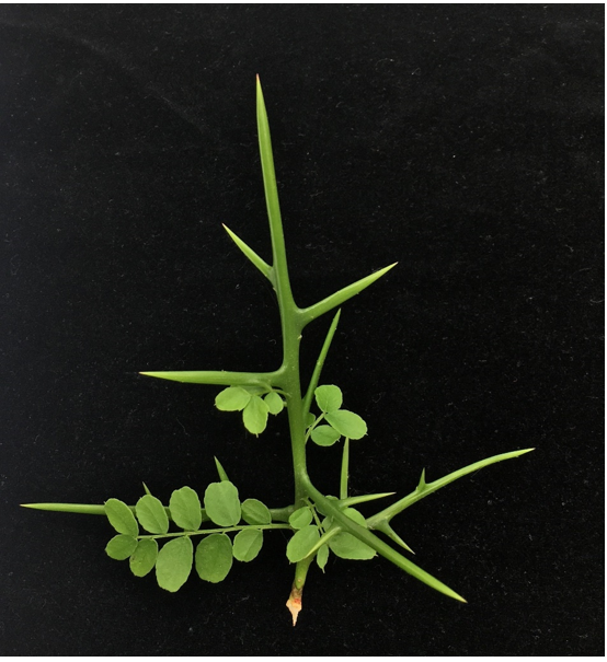
In the classic textbook “Patterns in Plant Development”, by Taylor Steeves and Ian Sussex, thorns are viewed as “one of the most striking departures from typical shoot morphology”. Our work serves as a first step for understanding how such evolutionary novelties arise. With the identification of citrus thorn identity TI genes and a previously undescribed TI–WUS pathway for stem cell regulation, we now have a handle to explore the upstream and downstream regulators involved in weaponizing plants. It is also worth mentioning that thorns have evolved multiple times, and can exhibit very striking departures from shoots, for instance as in honey locust thorns (Figure 2). It still remains to be seen if different plant species redeploy the TI-WUS pathway for thorn development, or if different species armor themselves in unique ways.
The Danish Stem Cell Center (DanStem) at Faculty of Health & Medical Sciences at the University of Copenhagen is looking for a Postdoctoral candidate to join the Aragona group starting November 2020 or upon agreement with the chosen candidate.
Background
The Novo Nordisk Foundation Center for Stem Cell Biology – DanStem has been established as a result of a series of international recruitments coupled with internationally recognized research groups focused on insulin producing beta cells and cancer research already located at the University of Copenhagen. DanStem addresses basic research questions in stem cell and developmental biology and has activities focused on the translation of promising basic research results into new strategies and targets for the development of new therapies for cancer and chronic diseases such as diabetes and liver failure. Find more information about the Center at http://danstem.ku.dk/.
A postdoctoral position is available in the group of Mariaceleste Aragona at DanStem. The team studies fundamental mechanisms of stem cell biology and tissue architecture establishment and maintenance. Our group aims to understand how neighbouring cells coordinate their decisions to build tissues with specialized structure and function. In particular, we want to investigate how mechanical cues affect gene transcription, stem cells dynamics and fate decisions. To achieve this, the group utilizes lineage tracing in mouse models, embryo tissue explants for live imaging during organ formation, transcriptomic and chromatin profiling at the single cell level. This research project will study the mechanisms by which the different compartments of the skin cope with mechanical stress, as well as how they coordinate their own homeostatic behavior with the different neighboring cell types. Starting date for this position is the 1 November 2020, or upon agreement with the chosen candidate.
Job description
We are seeking an enthusiastic and outstanding post-doctoral candidate with a strong background in either mouse and stem cell biology and/or molecular biology. The candidate will implement lineage tracing techniques and transcriptomic profiling to identify key cellular and molecular players regulating stretch-mediated tissue expansion in vivo. By combining clonal analysis to study cell fates dynamics, whole tissue imaging, single cell RNA sequencing and chromatin profiling, the candidate will master the underlying principles of tissue architecture maintenance upon mechanical perturbations.
Qualifications
Candidates must hold a PhD degree in cell/molecular/developmental/stem cell biology/ or similar, with a track-record of successful scientific work.
Candidates should have a strong background in mouse genetics, cell and molecular biology and/or cell imaging. Alternatively candidates with a background in transcriptomic applied to animal models are also encouraged to apply.
Previous experience using rodents as a research model, stem cell culture, embryo explants and/or next-generation sequencing and bioinformatics are considered an advantage.
Good English communication skills, both oral and written, are prerequisite for the successful candidate.
A solution-oriented, organizational and positive mindset is required. The ability to work in a highly collaborative environment both independently and as part of the team is essential.
Terms of salary, work, and employment
The employment is planned to start 1 November 2020 or upon agreement with the chosen candidate. The employment is initially for 2 years with the possibility for renewal. The terms of employment are set according to the Agreement between the Ministry of Finance and The Danish Confederation of Professional Associations or other relevant professional organization. The position will be at the level of postdoctoral fellow and the basic salary according to seniority. Currently, the salary starts at 34.650 DKK/approx. 4,.650 Euro (April 2020-level). A supplement could be negotiated, dependent on the candidate ́s experiences and qualifications. In addition a monthly contribution of 17.1% of the salary is paid into a pension fund.
Non-Danish and Danish applicants may be eligible for tax reductions, if they hold a PhD degree and have not lived in Denmark the last 10 years.
The position is covered by the “Memorandum on Job Structure for Academic Staff at the Universities” of December 11, 2019.
The application must include:
Motivation letter (It should describe your long-term research vision, the reason for applying to be part of our team and why you think you are the right candidate to fill this position).
Curriculum vitae incl. education, experience, previous employments, language skills and other relevant skills.
List of three references (full address, incl. email and phone number).
The application, in English, must be submitted electronically by clicking APPLY below.
The University of Copenhagen wishes to reflect the diversity of society and welcomes applications from all qualified candidates regardless of personal background.
Only applications received in time and consisting of the above listed documents will be considered.
Applications and/or any material received after deadline will not be taken into consideration.
The application will be assessed according to the Ministerial Order no. 284 of 25 April 2008 on the Appointment of Academic Staff at Universities.
Assessment procedure
After the expiry of the deadline for applications, the authorized recruitment manager selects applicants for assessment on the advice of the Appointments Committee. All applicants are then immediately notified whether their application has been passed for assessment by an expert assessment committee. Selected applicants are notified of the composition of the committee and each applicant has the opportunity to comment on the part of the assessment that relates to the applicant him/herself.
Application deadline: August 23, 2020, 23.59pm CET
Founded in 1479, the University of Copenhagen is the oldest university in Denmark. It is among the largest universities in Scandinavia and is one of the highest ranking in Europe. The University´s eight faculties include Health Sciences, Humanities, Law, Life Sciences, Pharmaceutical Sciences, Science, Social Sciences and Theology. www.ku.dk
The Danish Stem Cell Center (DanStem) at Faculty of Health & Medical Sciences at the University of Copenhagen is looking for a (AC-TAP) candidate to join the Aragona group starting November 2020 or upon agreement with the chosen candidate.
Background
The Novo Nordisk Foundation Center for Stem Cell Biology – DanStem has been established as a result of a series of international recruitments coupled with internationally recognized research groups focused on insulin producing beta cells and cancer research already located at the University of Copenhagen. DanStem addresses basic research questions in stem cell and developmental biology and has activities focused on the translation of promising basic research results into new strategies and targets for the development of new therapies for cancer and chronic diseases such as diabetes and liver failure. Find more information about the Center at http://danstem.ku.dk/.
Job description
The candidate will be responsible for purchasing and general stock maintenance for the whole group, which includes keeping track of orders, receiving, unpacking deliveries and approving invoices. He/she will maintain the laboratories protocols and stock database and will play a key role in tasks ensuring a good working order of the laboratory in collaboration with the other group members. He/she will also be assist in preparation of in-house reagents used by the laboratory and managing the team’s mouse colony.
In addition to these tasks, the candidate will assist in a research project in collaboration with post-doctoral fellows and/or PhD students. Such a project will be related to the study of stem cells dynamics and tissue architecture maintenance upon mechanical perturbation, and will involve the preparation of whole mounts for confocal imaging, sectioning and immunostaining of tissues, preparation of cell suspensions for FACS analysis and molecular biology, among others. The successful applicant is expected to learn new laboratory techniques and become able to use them autonomously. Furthermore, he/she will attend weekly seminars and laboratory meetings. The working hours are 37 hours per week.
For additional information about the position above, please contact Associate Professor Mariaceleste Aragona mariaceleste.aragona@sund.ku.dk
Qualifications
A Master’s degree or equivalent in a biological sciences-related discipline.
Highly motivated and enthusiastic candidates are encouraged to apply. The position requires solid previous work experience from an established research laboratory. Skills in several of the following techniques are required: mouse handling and genotyping, molecular biology (PCR, cloning), cryosectioning and immunocytochemistry. Experience in working with mouse models is a prerequisite for the successful candidate.
Knowledge of cell and tissue biology, stem cell biology or mechanobiology is an advantage.
The position requires good computer literacy and previous experience in a similar position will be a strong advantage.
The applicant should be reliable and well organized. A solution-oriented, organizational and positive mindset is required. The work requires independence and demands flexibility and accuracy. Further, you must have good interpersonal skills and interest in working in an international team.
Good English communication skills, both oral and written, are prerequisite for the successful candidate and Danish is desirable.
Terms of salary, work, and employment
The employment is scheduled to start November 1, 2020 or upon agreement. Contract is for 2 years.
The place of work is at the Novo Nordisk Foundation Center for Stem Cell Biology (Danstem), University of Copenhagen, Blegdamsvej 3B, Copenhagen.
Salary, pension and terms of employment are as Academic Research Staff (Akademisk medarbejder) in accordance with the provisions of the collective agreement between the Danish Government and AC (Danish Confederation of Professional Associations). In addition to the basic salary, a monthly contribution to a pension fund is added (17.1% of the salary).
The application must include
Motivation letter
Curriculum vitae incl. education, experience, previous employments, language skills and other relevant skills
List of three references (full address, incl. email and phone number)
The application, in English, must be submitted electronically by clicking on APPLY.
The University of Copenhagen wishes to reflect the diversity of society and welcomes applications from all qualified candidates regardless of personal background.
Only applications received in time and consisting of the above listed documents will be considered.
Applications and/or any material received after deadline will not be taken into consideration.
The Group of Nico Posnien at the Department of Developmental Biology of the Georg-August-University of Göttingen invites applications for a fully funded
PostDoc Position
starting from November 1, 2020 for the duration of one year. The salary is in accordance with the German public service salary scale (E13 TV-L) at 100% of the regular working hours (currently 39.8 hours per week).
Background and aim of the project:
We study the evolution of Drosophila head shape and compound eye size (e.g. see here) to contribute to a better understanding of the molecular basis of the morphological diversity. The PostDoc project will focus on interspecific differences in head development between D. americana and D. novamexicana and it builds on prior phenotypic and genetic data. The major aim of the project is revealing interspecific differences in developmental gene expression and chromatin accessibility using an already available extensive RNAseq and ATACseq dataset. Expression and accessibility data will be integrated with genome wide association mapping (GWAS) data (see here) to link variation in gene regulation to phenotypic differences. Additionally, the impact of various inversions that are present between D. americana and D. novamexicana (see here) on gene regulation and phenotypic differences will be tested.
Your profile:
PhD in Biology, Bioinformatics or related fields
Experience with Next Generation Sequencing (NGS) data is expected
Background in Bioinformatics, Statistics and strong analytical skills is expected
Experience with molecular biology (cloning, PCR) and/or Drosophila genetics is advantageous
What we offer:
The University of Göttingen is part of the interdisciplinary Göttingen Campus that offers a vital environment for basic research and a well-organized PostDoc community. The University of Göttingen is an equal opportunities employer and places particular emphasis on fostering career opportunities for women. Qualified women are therefore strongly encouraged to apply in fields in which they are underrepresented. The university has committed itself to being a family-friendly institution and supports their employees in balancing work and family life. The mission of the University is to employ a greater number of severely disabled persons. Applications from severely disabled persons with equivalent qualifications will be given preference.
Please send your application (motivation letter, CV, academic certificates and transcript of records, as well as contact information of 1-3 references) as a single pdf file to nposnie@gwdg.de.
We are seeking a highly motivated, organized and enthusiastic postdoctoral fellow or research associate to study embryonic kidney development and its relationship to developmental kidney diseases. We are interested in the role of Wnt signaling in shaping nephric tubules, utilizing Xenopus (frog) embryos and mammalian tissue culture as models. Current goals include: 1) Determining how junctions are formed during tubule formation; 2) Modeling how patient mutations result in human developmental kidney diseases; 3) Discovering novel components affecting nephron development; 4) Visualizing in vivo tube formation using advanced live imaging techniques; 5) Generating transgenic animals to visualize nephrogenesis in vivo
Current projects utilize developmental, molecular and cell biological approaches including imaging in living embryos. Applicants with a Ph.D., M.D. or equivalent and a strong background in Developmental Biology, Embryology, Cell Biology, Molecular Biology and/or Stem Cell Biology are highly encouraged to apply. Salary and benefits are commensurate with relevant experience. Review of applications will continue until the position has been filled.
Please send your CV, cover letter indicating current and future research interests, and the name/email address of three references to:
 (No Ratings Yet)
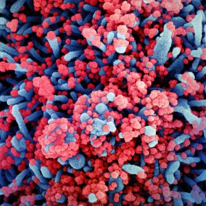 In the latest episode of Genetics Unzipped, Kat Arney looks at the ancient war between our genes and the pathogens that infect us, going back thousands of years to the Black Death and before, through to our very latest foe: the SARS-CoV-2 coronavirus behind COVID-19.
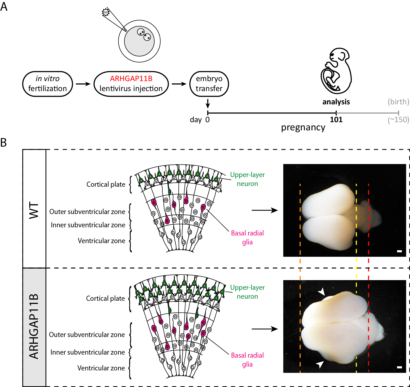
 (9 votes)
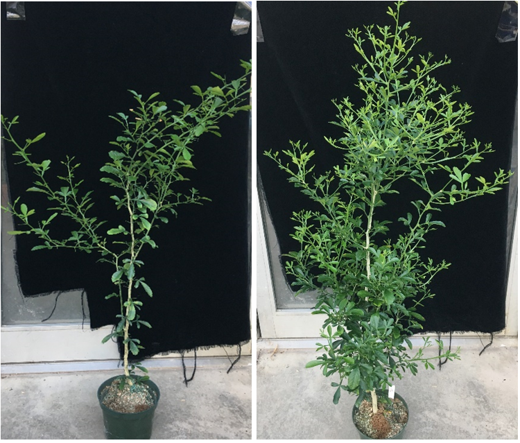
 (2 votes)