We are seeking highly motivated candidates to join us on a project beginning in 2019 on the molecular mechanisms of sensory neurogenesis. We study in particular the nociceptors, the specialized peripheral neurons that detect painful stimuli.
We aim to understand the role and mechanism of action of the Prdm12 gene. Prdm12 encodes an evolutionarily conserved epigenetic regulator of gene expression that has been found mutated in patients that suffer from a rare disease, Congenital Insensitivity to Pain, a dangerous condition that renders individuals completely unable to feel pain since their birth (Chen et al., Nat. Genet., 2015). To understand the molecular mechanisms that cause the painlessness, we are using the frog embryo and have generated Prdm12 null and conditional knock-out mouse models. We expect that the results of our work using these experimental systems as well as the identification of Prdm12 direct targets and interacting partners will help in the development of new strategies for treating pain.
The positions are funded by the Walloon government within the frame of the “Win2wal” program. They are open from 2 to 4 years and starting dates are flexible. The research will be performed in the laboratory of Developmental Genetics (Dr. Eric Bellefroid, http://gendev.ulb.ac.be/bellefroidlab/) that is part of the University of Brussels (ULB) Neuroscience Institute (UNI), the ULB Structural Biology and Biophysic laboratory (Dr. Abel Garcia-Pino, https://www.cm2ulb.be/) and the laboratory of Neuroscience (Dr. Laurence Ris, https://sharepoint1.umons.ac.be/FR/universite/facultes/fmp/services/neurosci/Pages/Equipe.aspx) at the University of Mons.
Preference will be given to applicants with a background in one of the following: mouse genetics, electrophysiology, cell and molecular biology and genome wide approaches (ChIP-seq,…).
Interested candidates should send a letter of motivation (before february 2019) describing past research experiences and full CV to:
Eric Bellefroid (ebellefr@ulb.ac.be), Laurence Ris (Laurence.RIS@umons.ac.be) or Abel Garcia Pino (agarciap@ulb.ac.be) together with the name and e-mail address of 2 references.
Selected related publications:
Thelie et al., (2015). Prdm12 specifies V1 interneurons through cross-repressive interactions with Dbx1 and Nkx6 genes in Xenopus. Development, 142(19), 3416-3428.
Nagy et al., (2015). The evolutionarily conserved transcription factor PRDM12 controls sensory neuron development and pain perception. Cell Cycle, 14(12), 1799-1808.
Written and illustrated by: Bjørt K. Kragesteen, Malte Spielmann, and Guillaume Andrey.
In early development, the forelimb and hindlimb buds of tetrapods are morphologically uniform. However, as limb development proceeds, each individual tissue attains a characteristic morphology that ultimately defines the identity of a forelimb (arm) or a hindlimb (leg). How do undifferentiated limbs bend their morphogenetic trajectories into arm and legs, since they are patterned by similar developmental processes? It is commonly accepted that the differential activities of a handful of genes instruct the formation of either arms or legs; yet the mechanism leading to their differential regulation in fore- and hindlimb buds was unknown. In our recent study, we dissected in detail such regulatory mechanisms and have revealed, once again, how important the function of the non-coding regulatory genome is, representing the overwhelming majority of vertebrate genomes.
In Stefan Mundlos’ research group at the Max Planck Institute for Molecular Genetics in Berlin, the focus is on the lessons that human limb malformations can teach us about gene regulation. Most research projects start with detecting the genomic mutation in human patients with congenital limb malformations at the Charité Berlin university hospital. These limb malformations are frequently caused by large changes in the DNA called structural variants including: deletions (removing information), inversions (displacing information), and duplications (doubling and misplacing information). One can imagine that such mutations might mess up the genetic information, and by detecting them in patient genomes, structural variants can provide a clue as to where important non-coding regulatory elements are located. From this starting point, it is possible to look for neighbouring genes that become misregulated following the mutation, ultimately changing the developmental program and the formation of the embryo.
Our story started back in 2010 when Malte Spielmann, a clinical scientist interested in structural variants and congenital disease, tried to work out the genetic cause in three families with a very rare malformation syndrome affecting the arms of the patients, known as Liebenberg syndrome (named after the doctor that first described it back in 1973). When he looked at the X-rays of the patients upside down, it struck him that the arms looked very much like legs! If we think about our arms and legs, they actually share many similarities: both are formed by one long bone (upper arm/thigh: the humerus/femur), followed by two bones (lower arm/leg: ulna/fibula and radius/tibia), terminating in many small bones (hands/feet: carpals, metacarpals, and phalanges) (see Figure 1).
Figure 1. Limb development: from buds to arms and legs. Arms and legs are serial homologs; notice their similarities as well as their specialised joints that enable specific functions.
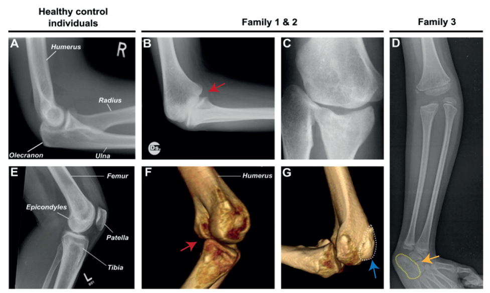
Nevertheless, they flex in opposite directions, as the arms have a specialised elbow joint, where the tip of the ulna called the olecranon (the pointy elbow) grabs around the distal end of the humerus. The legs have a specialised knee joint with a small bone, the patella (knee cap), ensuring stability and enabling weight bearing. However, the Liebenberg syndrome 3D CT scan showed the following: the fingers were very short (brachydactyly) looking very much like toes; the small bones of the wrist (pisiform, triquetral) were fused together looking like the heel bone (calcaneus), and the olecranon was reduced and no longer grabbing around the end of the humerus. Instead, the end of the humerus was broader as a patella like bone appeared fused to it (Figure 2).
Figure 2. Liebenberg syndrome: partial arm-to-leg transformation. A and E show healthy arms and legs, respectively. The rest show x-ray and CT-scan of patients with Liebenberg syndrome. Red arrow: elbow joint resembling a knee joint. Blue arrow: patella like bone fused on humerus. Yellow arrow: wrist bones fused resembling the calcaneus (heel bone).
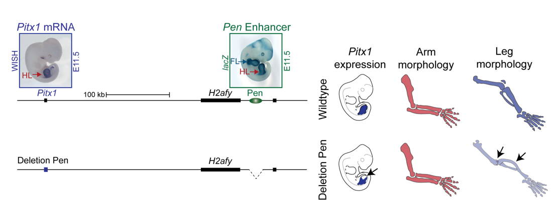
How on earth could this happen? Malte performed DNA analysis (array-CGH) and found a large deletion (107 kb) on chromosome 5 in all affected individuals. The deletions remove the gene H2AFY. However, this gene is a housekeeping gene and in mice in which the gene had been inactivated do not show any limb phenotype. Malte then looked on each side of the gene and found two interesting things:
On the centromeric side lies a gene named PITX1, which is expressed exclusively in the hindlimb during limb development and is known to be the only transcription factor that patterns the tissue. Inactivation of Pitx1 in mice results in reduction of leg morphology, such as loss of the patella and reduction of the calcaneus and the knee joint changing into an elbow-like joint. On the contrary, misexpression of Pitx1 in mouse forelimbs partially transforms the elbow joint into a knee like joint. Thus, Pitx1 misregulation in the forelimb seemed like a good candidate to explain to Liebenberg phenotype. However, Pitx1 regulation in tetrapods was unknown. Why would a deletion 200 kb upstream of the PITX1 promoter cause Liebenberg syndrome?
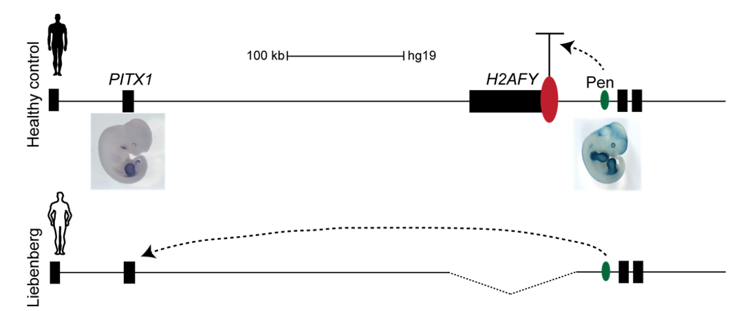
Interestingly, on the telomeric side of the deletion, 300 kb upstream of PITX1, a non-coding enhancer element can be found, called Pen (pan limb enhancer) that is active in both forelimbs and hindlimbs. Enhancer elements are defined as sequence specific stretches of DNA that are bound by transcription factors that dictate the activity and ensure communication with the correct gene promoters through chromatin folding. Often several enhancer elements regulate a target promoter and the collective activity of the tissue specific enhancer reflects the promoter transcriptional output. Recent development of proximity-ligation chromatin conformation capture technology (e.g. genome wide Hi-C) has demonstrated that the genome is partitioned into topological associating domains (TADs). TADs are scaffolds of preferential interactions between cognate promoters and enhancers and thus protect them from promiscuous activity from neighbouring TADs by boundary elements. These TADs were said to be stable across cell types and evolutionary conserved. With this in mind, the following hypothesis was formulated:
The Liebenberg deletion removes a TAD boundary element that normally separates PITX1 and Pen, resulting in PITX1 adopting a foreign enhancer, i.e. Pen, that is active in both fore- and hindlimbs. This enhancer adoption thus results in abnormal activation of PITX1 in the forelimb, where it should never be expressed, altering the patterning of the forelimb into a hindlimb, and partially transforming the arms into legs (Figure 3).
Figure 3. PITX1 locus in humans: Liebenberg deletion misplaces Pen enhancer. In control humans, PITX1 (expressed in hindlimb only) and Pen enhancer (active in fore- and hindlimbs) are 350 kb apart. In Liebenberg patients, large deletions bring Pen enhancer closer to PITX1 misexpressing the gene in forelimbs.
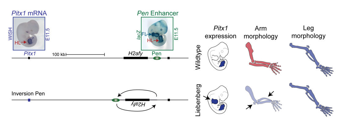
To test the hypothesis, Bjørt Kragesteen, a PhD student in the lab interested in deciphering non-coding functionality, sought to discern the molecular pathomechanism of Liebenberg syndrome together with Malte. First Bjørt created mouse mutants using CRISPR-Cas9 engineering that was newly established in the lab (back in 2013). She used two gRNAs to generate Liebenberg-like deletions and inversions at the mouse Pitx1 locus. Excitingly, analysis of Pitx1 mRNA expression in the early mutant mouse embryos showed Pitx1 misexpression in forelimbs! Skeletal analysis of adult mice showed a Liebenberg-like phenotype where the olecranon was reduced, an ectopic bone (patella-like) appeared at the humerus and the rotation of the arm was similar to the legs (Figure 4). Amazing. Case solved.
Figure 4. Pitx1 locus in mice: CRISPR engineered mice show partial arm-to-leg transformation. A 113 kb inversion misplacing Pen closer to Pitx1 resulted in its misexpression in arms and consequent partial arm-to-leg transformation with bowing of the radius and appearance of a patella-like bone (arrows).
However, many questions remained unanswered. Why is Pen, a strong fore-and hindlimb enhancer, located relatively close to Pitx1? Isn’t that too risky for a key hindlimb patterning gene?
In parallel to Bjørt’s project, Guillaume Andrey, who started his postdoc in the laboratory in early 2014, was investigating the normal regulation of Pitx1, by combining deletions and inversions of its putative regulatory landscape and enhancer assays. He observed that several engineered structural variants, which did not alter the pre-supposed boundary between Pitx1 and Pen, resulted in a mirror image pattern between fore- and hindlimb, identical to the one of the Pen activity and a Liebenberg phenotype. This observation suggested that Pitx1 could be controlled by the Pen element even when the “boundary” was intact. From that point, it became evident that in hindlimbs Pen could play a role in the regulation of Pitx1.
We thus next deleted the Pen enhancer to see what would happen. A visit to the animal facility some weeks later revealed that some of the adult homozygous Pen deletion mice developed club feet, dragging their hindlimbs behind. Both mouse and human patients haploinsufficient for Pitx1 develop clubfeet. Moreover, the mutants showed reduced Pitx1 expression and skeletal abnormalities whereby the patella was missing (Figure 5). This was solid evidence that Pen indeed is a Pitx1 enhancer!
Figure 5. Deletion of Pen results in reduction of Pitx1 expression and loss of hindlimb morphology. CRISPR engineered deletion removing Pen enhancer results in abnormal rotation and articulation of the knee joint and loss of the patella.
With this exciting finding we identified something not hereto described: A gene can be regulated by an unspecific long range enhancer; however, changing its location in the 2D regulatory landscape results in misregulation of the target gene and can transform tissue morphologies. We continued the search for a hindlimb specific Pitx1 enhancer, but no matter how much cloning and testing of enhancer elements we did, no hindlimb specific enhancer could be found. We thus decided to join forces, merging the projects about the normal and Liebenberg regulation of Pitx1, in order to understand how a gene that is solely expressed in the hindlimb can be controlled by unspecific enhancer elements active in both forelimbs and hindlimbs.
The research question thus became: what prevents Pitx1 expression in forelimbs in wildtype animals if its enhancer is active in both pairs of limbs?
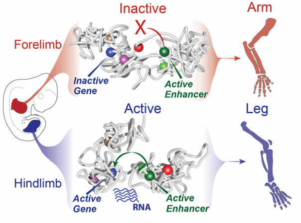
The next obvious layer of gene regulation to scrutinise was the chromatin folding at the Pitx1 locus in limbs. We first employed circular chromatin conformation capture (4C) technology in forelimbs vs hindlimbs to detect which regions surrounding Pitx1 were in close proximity to the gene. But, using the Pitx1 promoter region as a viewpoint, no differences were observed. However, Guillaume was using a slightly alternative 4C viewpoint in the gene body, and using the same library could see very strong differences between the tissues and clear Pitx1-Pen interactions in hindlimbs, indicating that the locus structure was highly defined. This was further confirmed using capture-C variation of the method using a larger fragment as a “bait” to see the interactions with the Pitx1 promoter region. Excitingly, differences between forelimbs vs hindlimbs emerged whereby Pitx1 showed differential interactions with Pen: in hindlimbs, Pen and Pitx1 come into close proximity enabling its tissue specific activation, while in forelimbs they are kept separated! Yet, this did not give the complete picture. At that point in time (2016) a new C-method, capture Hi-C, was developed and we established it in the lab. Here RNA probes are used to pull down a region of interest, and we enriched 3 megabases surrounding the Pitx1 locus. This provides a more complete picture of the interactions over the whole locus. Contrasting forelimbs and hindlimbs interaction heat-maps showed a clear difference: in hindlimbs Pitx1 forms loops with several regions (RA1, RA3 and Pen), which were almost completely diminished in forelimbs, but with a forelimb specific loop with the repressed gene Neurog1 occurs.
Still, this type of analysis gave us a 2D image of what was going on at the locus and we had a hard time imagining what this looks like in 3D, despite many hand drawn depictions. We thus initiated a collaboration with physicists in Italy in Mario Nicodemi’s research group. They used our capture Hi-C data and ran computational simulations using a so-called strings and binders model. They sent us the modelling results and 3D videos of forelimbs vs hindlimbs as well as an inversion mutant that shows the Liebenberg phenotype. The result was jaw-dropping: in wildtype forelimbs, the locus forms an inactive conformation whereby Pitx1 and Pen are kept a part, and where the repressed Pitx1 is embedded within its own domain next with repressed Neurog1 (neither of the genes are active in forelimbs and thus are covered with repressive epigenetic marks and hang out together). In wildtype hindlimbs, the locus folds in three domains and now Pitx1 is sitting at the surface of its domain directly facing Pen, thus enabling communication and robust transcription. Finally, in mutant forelimbs, bringing Pen closer to Pitx1 results in active folding of the whole locus, such as that in hindlimbs. Thus, not only do Pen and Pitx1 interact ectopically in mutant forelimbs, but the 3D-conformation becomes hindlimb-like, resulting in ectopic Pitx1 expression and arm-to-leg transformation.
Figure 6. Of arms and legs: dynamic chromatin folding of the Pitx1 locus ensures its correct regulation by Pen enhancer and normal morphogenesis. In forelimbs, Pitx1 and Pen are separated ensuring an inactive chromatin folding and absence of transcription ensuring normal development of arms. In hindlimbs, Pitx1 and Pen are facing each other resulting from an active folding of the locus leading to robust Pitx1 expression and normal leg development.
With all these data in hand and the genetic evidence that Pen was responsible when misplaced in the nuclear 3D space for the ectopic expression of Pitx1 in the “Liebenberg” forelimb, we could determine that the Pitx1 locus dynamic structure modulates the Pen activity in normal embryos. Specifically, in forelimb it represses the enhancer by keeping it away from Pitx1 promoter and that upon activation in hindlimb, it can participate in Pitx1 robust expression. Finally, it also showed that ectopic interaction between a gene and its own enhancer, following structural variant, in a process called gene endo-activation can cause gene misexpression and disease.
Read the full story:
Kragesteen B.K.*, Spielmann M.*, Paliou C., Heinrich V., Schöpflin R., Esposito A., Annunziatella C., Bianco S., Chiariello A.M., Jerković I., Harabula I., Guckelberger P., Pechstein M., Wittler L., Chan W.L., Franke M., Lupiáñez D.G., Kraft K., Timmermann B., Vingron M., Visel A., Nicodemi M., Mundlos S. and Andrey G.
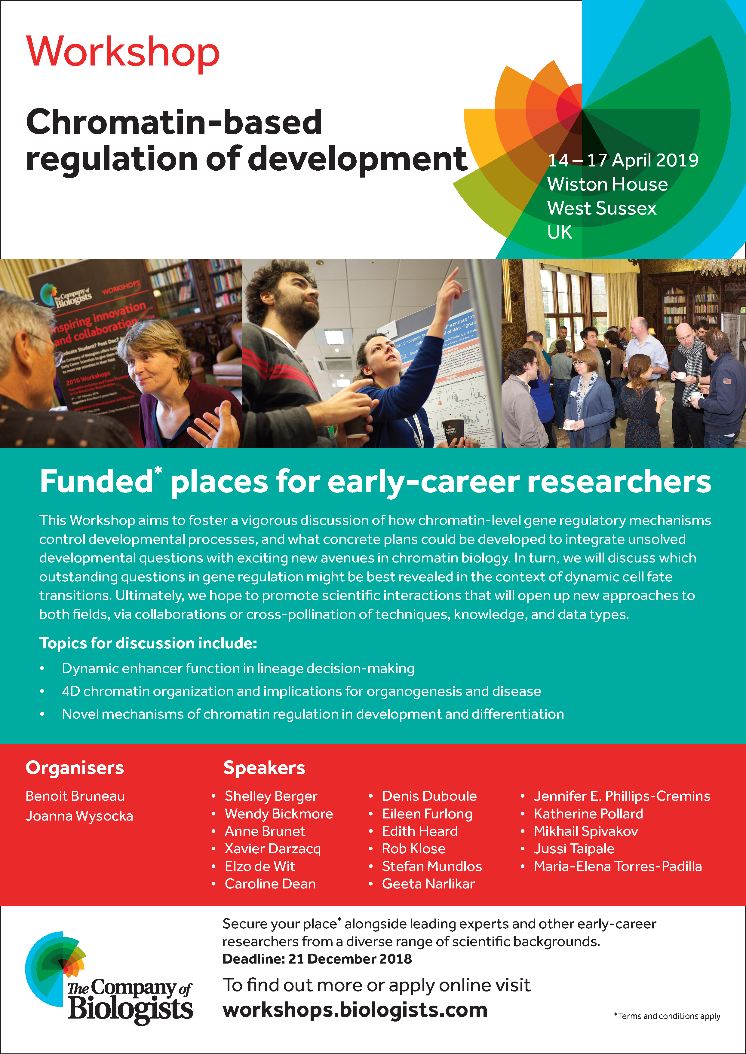
In April 2019, The Company of Biologists Workshop ‘Chromatin-based regulation of development‘ will be held in Wiston House, a 16th century Grade I listed building located at the foot of the South Downs in West Sussex.
Organised by Benoit Bruneau and Joanna Wysocka, the workshop will foster discussion of what mechanisms related to chromatin biology are informing developmental processes, and which outstanding questions in gene regulation might be best revealed in the context of dynamic cell fate transitions.
If all of this sound tantalising to you, there are around 10 funded places available to early career researchers. It’s an amazing opportunity for young researchers to participate in a relatively small (~30) group of world leading experts from across the field of gene regulation.
Deadline for applications is 21 December 2018.Find out more here:
In September, Development held the third of its highly successful series of meetingsfocusing on human developmental biology. Here at the Node we ran a competition to find a meeting reporter who would share their experiences of the meeting in exchange for free registration. Competition winner Antonio Barral Gil, a PhD student in Miguel Manzanares’ Lab at CNIC (The Spanish Center for Cardiac Research) in Madrid, now recollects an enriching few days in the heart of the English countryside.
Antonio in the lab
We, the scientists of all disciplines, are in a unique position in the world. While our work is most of the time very labour intensive and solitary, we must continuously rely on the rest of the community in order to both grow ourselves and to contribute to the advance of common knowledge, which itself will eventually feed back to us. It is this interconnection between the individual and the communal that I find the most beautiful thing in science. The fact that it is built upon sharing makes it one of the most human (or should I say, humane) areas of work one could think of. Meetings like Development’s “From stem cells to human development” are a testament to this. It was truly an enriching and exciting opportunity to be able to interact with people so committed to their work, so selflessly giving their lives to a cause that is ultimately poured back into our society, and even more beneficial to me considering I am just starting my scientific career.
Wotton House, the conference venue
The surprisingly sunny and pleasant English countryside that welcomed us was in line with the general mood of the meeting. At an outstanding venue, loads of unpublished data on an extensive array of research topics were generously shared, which all came to stress the importance of human-based research in the current state of developmental biology. Despite the diversity of themes discussed, one could see two main sides to this meeting: one focused on unravelling the developmental mechanisms that take place in the human embryo, and another aiming to replicate them (both for basic and translational purposes) in the dish.
A journey into the embryo
Within the first group, we were very fortunate to have Alain Chédotal who together with other researchers is putting huge effort into imaging the human embryo. By developing and improving techniques that make embryos transparent, they are able to perform whole-mount inmunostaining with widely used antibodies, and then scan them completely using light sheet microscopy. This allows them to look, in an organ-by-organ or tissue-by-tissue fashion, through astonishingly beautiful images of the human embryo. Connected to this was the work of Antoon Moorman, who elaborated on the already well-known three-dimensional atlas that he and his group built based on the Carnegie collection of human embryos, with the purpose of generating an incredibly useful didactic interactive tool.
The several visual analyses presented were very well complemented by Laurent David’s talk, who is coupling single cell RNA-seq with time-lapse imaging to stage early human embryos in a precise way. This allows him to couple changes in gene expression in each region of the embryo with developmental time. We also heard about Alexander Meissner’s work on methylation of CpG islands, which surprisingly shows how the methylation profile of extraembryonic tissues is very similar to that of cancerous cells.
Out of the embryo, into the dish
The other side of the meeting showcased the huge effort many groups are putting into reproducing human development in vitro. The elegant micropatterns utilised by Ali Brivanlou and Aryeh Warmflash, as well as the intriguing gastruloids developed by Alfonso Martínez Arias, shed light onto the early phases of human development, the ones that are harder to study for obvious reasons. Additionally, we heard about how a plethora of organoids is being obtained with levels of specification never reached before. Several speakers stood out for me, including James Wells (who has managed to derive colonic organoids with such a level of complexity they even contain hematopoietic cells), Paola Arlotta (whose brain organoids are getting more and more complex with every tweak to their protocols, to the point they even obtain photosensitive neurons), and Matthias Lutolf (who uses microfluidic chips to develop intestinal organoids which become incredibly well self-organized and compartmentalized).
A breath of fresh air
Being in the first year of my PhD, it was especially encouraging to see so many speakers that were PhD students or postdocs, and how engaging their work was. For starters, Teresa Rayon (a postdoc in James Briscoe’s lab) is tackling a fundamental yet poorly understood process: how is time encoded in the genome? Using spinal cord motoneurons derived from either mouse or human pluripotent stem cells as her model, she is developing elegant experimental designs that promise to expose the mechanisms behind the process. Another completely different question, but just as exciting for me, is being approached by Elisa Giacomelli, who is trying to obtain more mature cardiomyocytes derived from induced pluripotent stem cells by co-culturing them with cardiac fibroblasts in spheroids.
Moreover, Belin Selcen Beydag-Tasöz, from Anne Grapin-Botton’s lab, presented exceptional work (published very recently in Development) which characterized in depth human fetal pancreas and endocrine progenitors, as well as more mature cell-types. The use of single-cell transcriptomic analyses allowed them to untangle the events that take place during endocrine specification in the human embryo, which they also compared to cells derived in vitro to study the similarities and differences between those and the in vivo processes. Last but not least, Blair Gage, a postdoc working at Dr. Gordon Keller’s group, started his talk with a simple yet accurate statement: to cure liver diseases, livers for transplants are required. In order to push towards the ultimate objective of obtaining complex, functional livers originating in the lab, he is focused on differentiating liver sinusoidal endothelial cells (LSECs), critical for the correct performance of this organ, from human pluripotent stem cells.
Several more pages could be filled with the rest of the brilliant presentations given, which ranged from primordial germ cell differentiation to pluripotency and X-chromosome inactivation, passing through neural differentiation and its involvement with disease, retina morphogenesis, the segmentation clock, and so on. Such a variety of topics shows how rich and exciting the human development field is nowadays.
Over a hundred developmental biologists gathered in Surrey for the meeting
The people, beyond the science
This kind of meeting would not be the same without the time outside the talks and the situations you find yourself in. After the quite intense sessions, the moments in which you finally get to unwind arrive, and with them the opportunity to get to know the minds behind the works presented. During the poster sessions, over a glass of wine or beer or a cocktail, as well as through the comforting dinners and the late night drinks, I was very privileged to be able to talk about both science and extra-scientific topics with a bunch of talented, keen scientists; some conversations, for sure, will be of help in my own work back at my lab in Madrid.
Naturally, I could not end without highlighting the great job the organisers did to end up with such a great line up of speakers: Paula Arlotta, Ali Brivanlou, Jason Spence and, of course, Olivier Pourquié, who handed over the baton to James Briscoe as the new Editor-in-Chief of Development at the final dinner of the meeting. I am also very grateful to the team at Development, not only for having given me a great opportunity to attend the meeting as the reporter for The Node, but also because I sincerely think the time and effort they put in coming up with the meeting was extraordinary: Nicky Le Blond, Joanna Berry, Seema Grewal, Katherine Brown and, especially, Aidan Maartens, Community Manager of the Node and Online Editor of Development, as he made my experience so much more comfortable and easier than if I would have been by myself.
The broad display of research topics, coupled with their novelty, great communication on part of the speakers and the effort made by the organizers so that all could run smoothly, made this meeting a great example of what modern science means at its core: honesty, inquisitiveness, creativity, perseverance, and, above all, cooperation.
The grounds of Wotton House on a cold clear morning
More lawns and trees
A fountain and some columns in the Italian Gardens
Morning mist
Attendees gather for an afternoon walk around the nearby countryside…
…up hill and down dale…
…past quaint cottages…
…serenely still ponds…
…trees starting to turn their colour…
…and a waterfall
Dinner on the final night…
…where discussion continued unabated
Development’s new Editor-in-Chief James Briscoe talks about his hopes for his new role…
…while outgoing EiC Olivier Pourquie says his goodbyes
Photo gallery by Aidan Maartens
Development’s next human-focused meeting is scheduled for 2020 – we’ll be running another meeting reporter competition so watch this space!
Newborn babies are a symbol of immense potential, as they can grow up to be become virtually anybody, from an astronaut to the president. It is no secret that throughout life, there are critical junctions in which specific events or decisions can direct us on one path or another. Such events occur in our brains; during embryonic development neurons are born and establish connections with each other creating a network, which serves the initial needs of the system but is often vastly different from the final, adult network. This preliminary network undergoes remodeling during the first years of life, and again during puberty, to refine the network connectivity to better suit our changing needs. You can imagine that much like a computer, it is enough to have one pair of wires crossed to wreak havoc on the entire system, and indeed defects in pruning have been suggested to be causal for neuropsychiatric conditions, such as Alzheimer’s, schizophrenia, and autism.
The refinement process is defined as the phenomenon in which exuberant connections that were formed during early developmental stages are selectively eliminated at later stages and often further refined by regrowth toward adult specific targets. This process occurs in a very stereotypical and timely manner in each individual. There are several mechanisms by which the nervous system can ‘tweak’ its connectivity, and these regressive events occur on different scales, from single synapses up to the elimination of entire dendritic or axonal processes while the cell body remains intact.
We study these processes in the fruit fly Drosophila melanogaster. One well studied example of remodeling neurons, in the fly, is that of the mushroom body (MB) ɣ neurons. During the larval stages, the MB ɣ neurons extend primary processes to form a small dendritic tree, termed the calyx, and then extend bifurcated axons to form two distinct, medial and dorsal, lobes. During metamorphosis, the dendrites are pruned completely and the axons are pruned up to the branch point; subsequently MB ɣ neurons regrow their axons and dendrites to form adult-specific connections which are distinct from those of the larva.
The MB structure is comprised of both intrinsic neurons (ɑ/β, ɑ’/β’ and ɣ also collectively known as Kenyon cells – KCs) and extrinsic neurons (MB output neurons (MBONs), modulating neurons, etc.), and has a well described role in associative olfactory learning and memory both before and after metamorphosis. While there has been considerable progress in understanding how the intrinsic MB ɣ neuron remodel in terms of the molecules involved and the cellular processes employed, not much is known regarding other extrinsic neurons of the MB circuit, or if the circuit undergoes remodeling as a whole.
Flies have two morphologically distinct life stages, larval and adult, separated by metamorphosis. This puts us in a unique position to identify neuronal circuits which establish functional yet distinct connections both before and after metamorphosis. Do these neurons coordinate their remodeling to establish functional connectivity in both stages of Drosophila life, and if so, how?
In the lab of Liqun Luo in Stanford, a postdoctoral fellow, Xiaomeng Milton Yu, and a PhD candidate, Dominic S. Berns, were looking for a model to study neuronal remodeling at the circuit level. They came across a unique neuron, the Anterior Paired Lateral (APL), which innervates the adult MB structure in a very intricate manner. They used sophisticated genetic tools to show that it too underwent remodeling, in a similar timeframe as the MB ɣ neurons. Unfortunately, at that time, there were no adequate tools to study these neurons, so the project was left to “sit on the shelf”. When Milton left the lab, he and Liqun shared their findings with Prof. Oren Schuldiner, also a Lou member alumnus, for the possibility of continuing the study.
When I joined the Schuldiner lab for my PhD, around the end of 2014, I was presented with this project as an optional project for my graduate studies. I immediately fell in love with it, and began contemplating on mechanisms through which different types of neurons could coordinate their development. My initial hunch was that these neurons, which classically communicate through neuronal activity and neurotransmitters, could somehow use the same communication mechanism to coordinate neuronal remodeling.
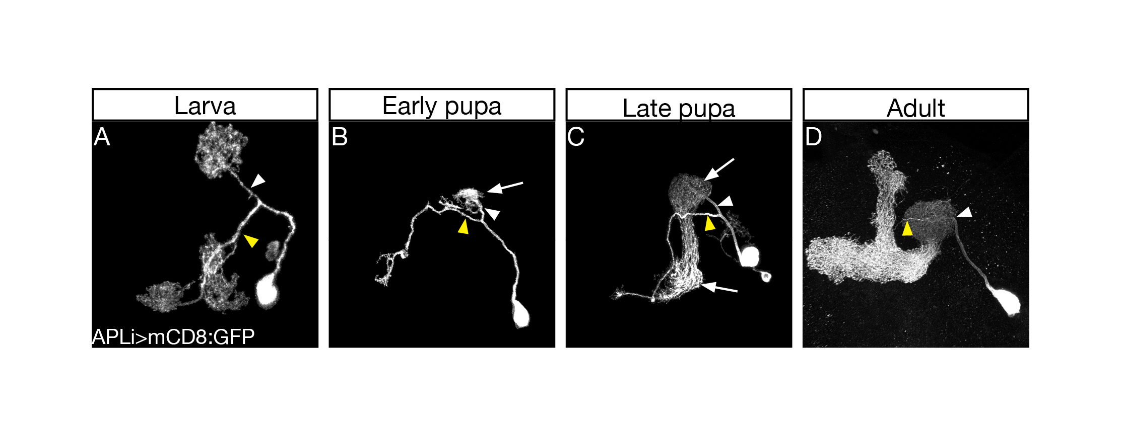
The first thing I started doing, as a novice fly person, was to scan for tools, essentially going over many Gal4 driver lines in search of one that would allow genetic access to the APL neurons throughout development. Many of the so-called APL specific drivers exhibited no, or inconsistent, expression during larva. Luckily for me, however, a very nice paper had just been published (Lin et al., 2014)from the lab of Gero Miesenböck in Oxford, about the APL neuron. In this work the first author Andrew Lin generated a new driver line which labelled the APL in the adult in a very clean and striking manner. Andrew was nice enough to send over the flies, and soon after receiving them I characterized their developmental expression pattern and was delighted to notice that they labelled the APL neurons throughout all stages of development (Figure 1).
Confocal Z projections of brains at 3rd instar larva (A), early pupa (B), late pupa (C), and adult (D), expressing mCD8::GFP driven by the APLi-Gal4. Yellow and white arrowheads mark the primary processes entering the MB dorsal lobe and calyx, respectively. White arrows indicate the regrowing APL. From Figure 1 in Mayseless et. al. 2018
Once I had found a good driver line highlighting the APL neuron throughout development, I started vigorously characterizing its development morphologically and molecularly. I quickly corroborated the initial findings that the APL undergoes remodeling in a similar timeframe as MB ɣ neurons. I then decided to test whether Ecdysone, the molting hormone in insects which was known to be a master regulator of neuronal remodeling, was also required for APL remodeling. As expected, when I inhibited Ecdysone signaling in the APL neurons and examined them during metamorphosis I saw unpruned APL neurites, indicating the requirement of Ecdysone signaling for APL pruning. When we examined these APL neurons at the adult stage, we were a little struck by what we saw, as the APL neurites which usually innervated the adult MB ɣ lobe were totally absent, while all other processes of the APL had regrown normally. This result puzzled us for a long time, and only after our initial submission of the paper for publication did we buckle down and analyze this phenotype. We hypothesized that the pruning and regrowth of the APL responded independently to Ecdysone signaling and set out to answer this question by inhibiting Ecdysone signaling in the APL only after pruning has occurred. This short side trip proved to be extremely interesting, as we found that not only are APL pruning and regrowth independently controlled by Ecdysone signaling, but that this differential control is probably regulated by different Ecdysone receptor isoforms.
After we had established that the APL and MB ɣ neurons, that form both pre and post synapses between them and thus form a mini-circuit, undergo remodeling, we set out to examine our original hypothesis: whether or not the remodeling of these neurons is coordinated and if so, how.
For this we planned on conducting two types of experiments; one would be where the APL neuron is missing or its pruning inhibited, and the other would be where the MB ɣ neurons are missing or their pruning inhibited. As we already had tools to manipulate the APL neuron while visualizing the MB ɣ neurons, we started with this set of experiments. Unfortunately, killing the APL neuron or inhibiting its pruning had very little to no effect on MB ɣ neurons.
At that point we did not have a good way to manipulate MB ɣ neurons while visualizing APL development. Lucky for us, at this stage of the study, the lab of Chris Potter was working hard on developing new tools based on their QF-QUAS system. The QF-QUAS system is a parallel binary expression system, very similar to that of the conventional Gal4-UAS, and permits independent genetic manipulation of two distinct populations. This tool set was exactly what we needed and Chris’s lab was generous enough to generate a QF2 based MB ɣ driver for us. Armed with these new tools we set out to undertake the second arm of our plan, to inhibit the pruning of MB ɣ neurons and examine the development of the APL neurons.
Upon conducting these experiments, we found that in animals in which we inhibited the pruning of MB ɣ neurons, the APL remodeling was significantly inhibited despite the fact that they were genetically untouched. These results indicated that our initial hypothesis was correct and that a coordination mechanism does exist! (Figure 2 top panel).
At this stage, we thought we had a nice descriptive paper and we set out to send the project for publication. While our reviewers agreed that it was interesting, they refused to accept our work and pushed us to examine how this coordination occurred.
Nonetheless, we were not deterred and fueled by our exciting findings we set out to test the second part of our hypothesis: is neuronal activity used to coordinate between remodeling neurons?
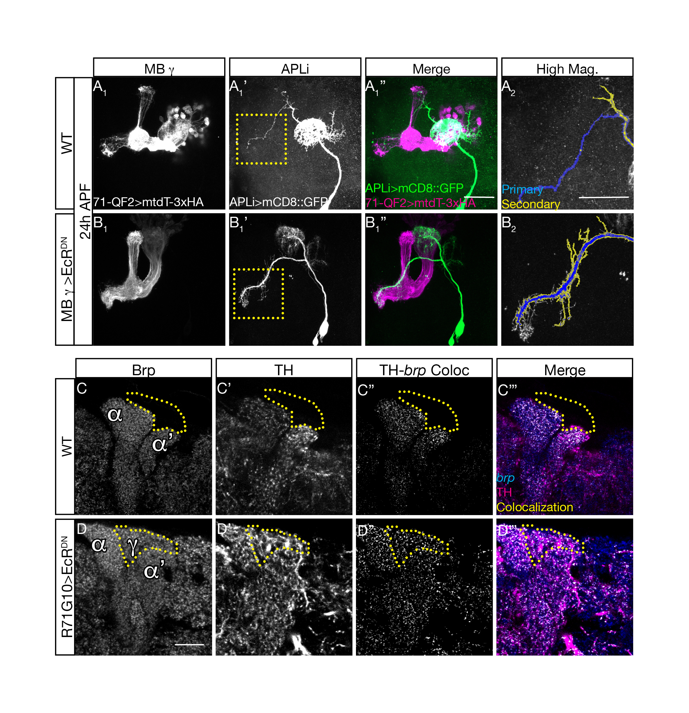
(A-B) Confocal Z projections of 24h APF WT brains (A) or those additionally expressing EcRDN in the MB g neurons (B). EcRDN expression was driven by 71G10-QF2G4H (Lin & Potter 2016). APL neurons were labeled by the APLi-Gal4 driving the expression of mCD8::GFP (gray in A1’-B1’, A2-B2, and green in A1”-B1”). MB g neurons were labeled by 71-QF2 driving mtdTomato-3XHA (magenta). Dashed boxes represent areas that are shown in high magnification in A2-B2 and which were segmented into primary (blue) and secondary (yellow) branches. (C-D) Confocal slices of adult WT brains (D) or those expressing EcRDN in MB g neurons driven by 71G10-Gal4 (D), additionally stained for Bruchpilot – Brp (gray in C-D and blue in C’’’–D’’’), Dopaminergic neurons marked by TH (gray in C-D’ and magenta in C’’’-D’’’). Colocalisation between TH and brp staining (gray in C’’-D’’ and yellow in C’’’-D’’’). Dotted outlines indicate ectopic or presumptive larval unpruned MB g neurites. From Figure 3 and 5 in Mayseless et al, 2018.
In order to test whether neuronal activity is involved we inhibited MB ɣ pruning but at the same time also inhibited MB ɣ neuronal activity. Remarkably, this uncoupled the development of the APL from MB ɣ and “allowed” the APL to undergo proper pruning even in the presence of unpruned ɣ neurons. We then wanted to ask what was the responding molecular mechanism in the APL, and tested whether Ca2+-Calmodulin nuclear signaling, a mechanism previously shown to play a prominent role in neuronal activity mediated ‘neuroprotection’, was involved. It was! Inhibiting nuclear Ca2+-Calmodulin signaling in the APL while inhibiting MB ɣ pruning had also uncoupled their development. Together, these results corroborated our initial hypothesis almost entirely. Not only are remodeling neurons capable of coordinating their remodeling but neuronal activity and Ca2+-Calmodulin signaling play a major role in this coordination.
Finally, we wanted to understand what is the meaning of this coordination for the adult animal. Does the inhibition of MB ɣ pruning influence the morphology of the APL at the adult stage? Is this the only neuronal population affected? Do they establish functional synaptic connections? We therefore examined the APL neurons as well as dopaminergic and serotonergic neuronal populations at the adult, all of which appeared to not only change their morphology in response to the inhibition of MB ɣ pruning, but also to form potentially functional synaptic connections with these unpruned larval MB ɣ neurites (Figure 2 bottom panel).
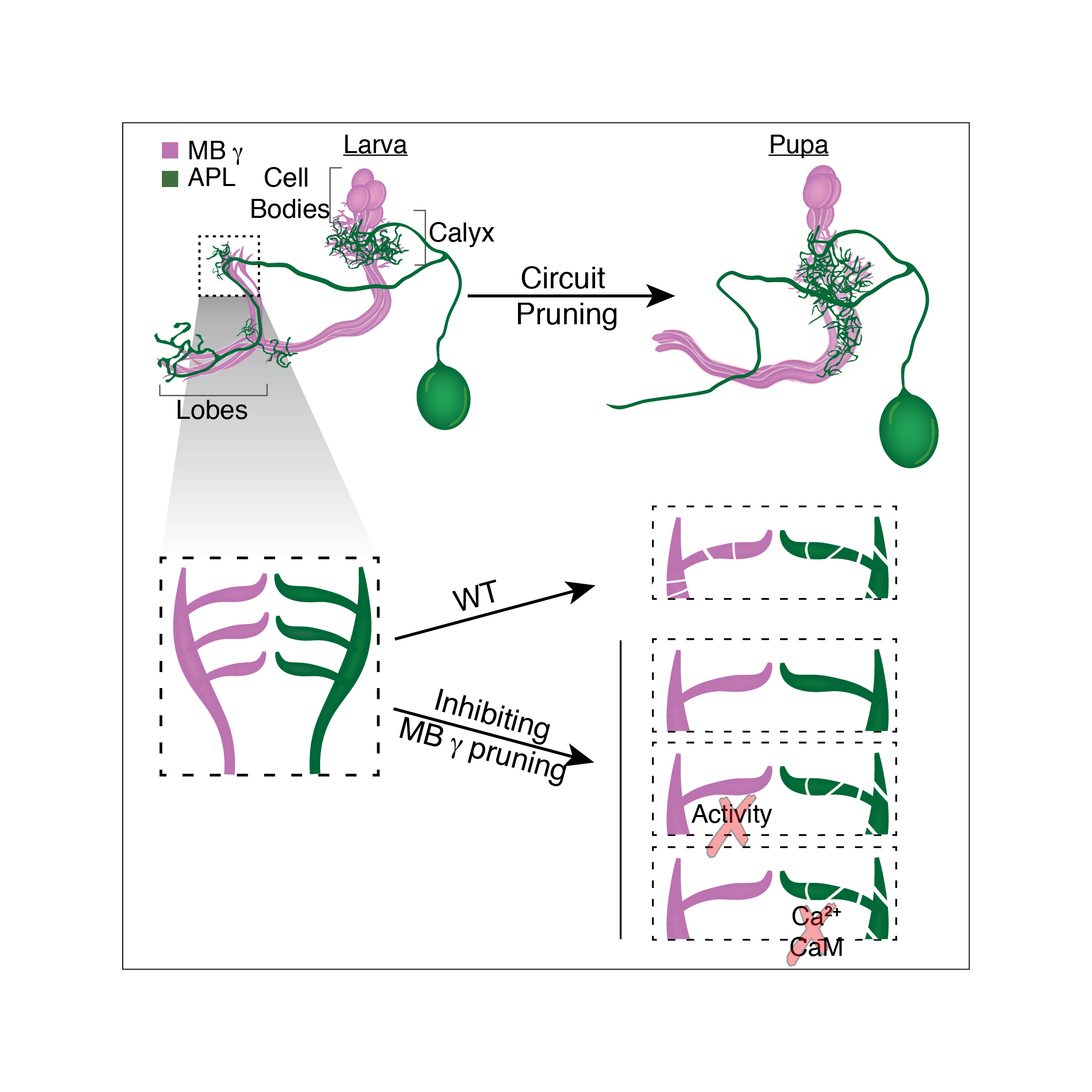
Schematic model outlining the findings in Mayseless et. al.,2018
In summary, our data suggests that miswiring of one neuronal type may have profound implications on the general connectivity of the adult nervous system. Extending these findings into humans, suggests that even a relatively minor defect in remodeling of specific neuronal populations may change the circuit in a substantial manner and result in a system-wide defect which could underlie potential pathological conditions, such as Alzheimer, schizophrenia or maybe even autism.
We are recruiting motivated and talented postdoctoral fellows to fill NIH-funded research positions in the Deans laboratory at the University of Utah. Our lab focuses on the contribution of Planar Cell Polarity (PCP) signaling towards multiple aspects of Inner Ear development in the mouse. We apply basic developmental biology, mouse genetics, and biochemical approaches to uncover key aspects of sensory hair cell differentiation and innervation. One of the following research projects could be yours: (i) transcriptional regulation of hair cell development and polarization, (ii) PCP signaling and axon guidance during cochlear innervation, or (iii) mechanisms of tissue patterning that guide planar polarity.
We are located in a highly dynamic research environment hosted by the Department of Neurobiology & Anatomy and share close ties with the Division of Otolaryngology. In addition, Utah provides unparalleled lifestyle and outdoor recreation opportunities for a superior work/life balance. Candidates should carry a PhD in the areas of developmental biology or neurobiology.Emphasis will be given to candidates with expertise in nervous system development though researchers using other developmental systems are encouraged to apply. Initial terms of appointment are for one year, with the expectation of renewal based on satisfactory performance and funding. Salary will be commensurate with prior research experience and NIH guides.
For consideration send a CV and list of references to Michael Deans, PhD (michael.deans@utah.edu).
The Department of Biology at Virginia Commonwealth University invites applications for three tenure-track faculty positions at the level of Assistant Professor to begin August 2019.
We seek candidates that use a variety of experimental approaches, model systems, and/or “-omic” technologies to investigate the molecular and cellular mechanisms of human disease. Candidates whose research focuses on the molecular basis of addiction are encouraged to apply.
Candidates are expected to develop a strong and creative research program and participate in undergraduate and graduate education. Successful applicants will have excellent opportunities to establish strong collaborations with researchers in the Department of Biology, the College of Humanities and Sciences, the VCU Medical Campus, School of Life Sciences, and Biomedical and Chemical Life Science Engineering. Applicants should have a PhD degree, and appropriate post-doctoral research experience to establish an independent research program and obtain extramural funding, a strong record of scientific achievement.
Virginia Commonwealth University, an urban R1 university in the heart of Richmond, Virginia, has an enrollment of approximately 32,000 undergraduate, graduate, and first professional students, including 43% minority, 29% underrepresented minority, and 1,452 international students from 101 countries. The university is recognized as one of the best employers for diversity and is committed to the recruitment and success of culturally and academically diverse faculty that reflect our unique campus demographics. The Department of Biology (https://biology.vcu.edu)has 44 full-time faculty members with diverse research interests in Cell and Developmental Biology, Evolution, and Ecological Processes and Applications, that teach and mentor over 2,000 undergraduate and over 45 graduate students. The Department has outstanding facilities and support, including a confocal microscopy suite, next-gen sequencers, and animal vivaria. In addition to an M.S. program, the Department is served by a doctoral graduate program in Integrative Life Sciences that provides five years of student support.
Please apply online at www.vcujobs.comand be prepared to submit a cover letter, curriculum vitae, a statement of teaching (1 page) and a statement of research accomplishments and plans (4-5 pages). You will be asked to list names and email addresses of three references. An email will be sent to your references, asking them to upload a letter of recommendation. The positions are open until filled. Priority consideration will be given to those applicants who apply by December 3rd, 2018.
Virginia Commonwealth University is an equal opportunity, affirmative action university providing access to education and employment without regard to age, race, color, national or ethnic origin, gender, religion, sexual orientation, veteran’s status, political affiliation or disability. Women, minorities and persons with disabilities are encouraged to apply.
In the Larsen lab, we are interested in testing a 50-year old question: How do sex combs rotate in fruit flies? Despite extensive studies of the process using 4D confocal microscopy, there remain many questions about the spatial and temporal dynamics of sex comb rotation we cannot address with currently available tools. We therefore turned to computer simulations and mathematical modelling to explore these issues.
It was love at first sight. JNM: I came to the University of Toronto with a strong interest in understanding how physical forces influence the evolution of morphogenesis. My PhD supervisor, Ellen Larsen, showed me a perfect model to explore this biological question: sex comb rotation. Although I was a bit skeptical because I did not know what a sex comb was and did not have any experience working with fruit flies, she convinced me in less than one minute. To do so, she showed a time-lapse movie of the rotating comb made by the other student in the lab, Joel Atallah (Mov. 1A). I was so intrigued by the beauty of this morphogenetic process, it was love at first sight.
Movie 1. Sex comb rotation. A) Time-lapse movie B) simulation. Early (red polygons) and late cell expansion (blue polygons). Rotating comb (green polygons), epithelial cells above the comb (yellow polygons).
Our hands were tied. This movie shows the development of the fore leg epithelium and embedded within it, a rotating row of bristle cells, the sex comb (Mov. 1). Thanks to the genetic tools available for fruit flies, we imaged combs of different lengths and angles of rotation. After a few years of hard work, we proposed that the driving force for the rotation came from a push from the epithelial cell growth underneath the sex comb1. However, to study cell growth in local areas and at different times was impossible with available biological techniques. Although our hands were tied using experimental biological tools, computer simulations set us free to explore the development and evolution of this morphogenetic process. To give you more insight into the comb rotation problem, here is some background information.
What are the sex combs of fruit flies?
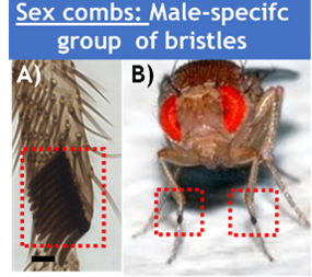
Sex combs are male-specific group(s) of bristles located on the front legs of many Drosophila species (Fig. 1).
Figure 1. Sex combs of Drosophila melanogaster. Adult sex combs are enclosed in red boxes. B was modified from reference 4.
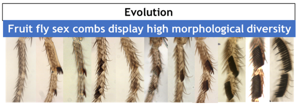
This row of bristles is used during courtship behavior, increasing the quantity of successful matings. As with any sexual trait, sex combs display an incredible morphological diversity among Drosophila species (Fig. 2).
Figure 2. Morphological variation observed among Drosophila combs.
Why study sex comb rotation? Despite the rapid progress achieved in understanding the genetic basis of evolution, the cellular basis remains much less studied. Sex combs are a great tool to investigate the cellular basis of evolution. Biologists including in our laboratory have used sex combs to study the developmental mechanisms underlying biodiversity1 and the cellular basis of allometric evolution2. Our present work shows an example in which mechanical forces play a fundamental role in understanding the evolution of morphogenesis.
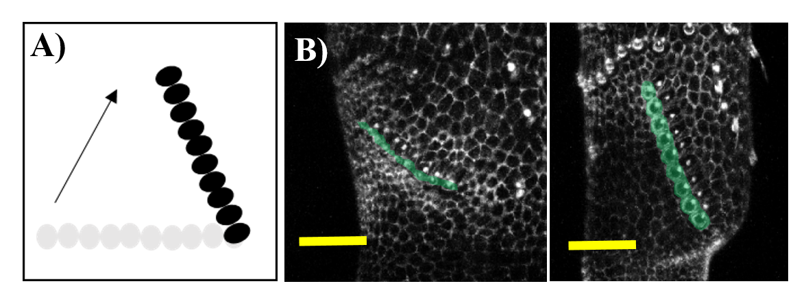
Figure 3. Sex comb rotation in Drosophila melanogaster. A) Schematic and B) Confocal images. In A, initial (gray circles) and final (black circles) sex comb position. In B, sex comb is shaded in green in B.
A bit of history. The study of sex comb rotation commenced in 1962 when Chiyoko Tokunaga, using genetic mosaics produced in sex combs during different times in development, hypothesized that this group of bristle cells changes in position during development3 (Fig 3A).
Our laboratory has concentrated on developing and standardizing an in vivo imaging technique to study comb rotation. To investigate the cellular mechanisms involved, we combine this imaging technique with standard genetic tools available for studying fruit fly morphogenesis such as mutants, transgenic flies with fluorescent proteins and artificial selection. Our work led to three candidate models concerning the source of the force underlying rotation (Fig. 4).
The one which hypothesizes the source of pushing force coming from the region distal to the sex comb (the “push” model) appears to best explain existing experimental data.
Figure 4. Hypothetical models of sex comb rotation. At least three hypothetical models can reproduce the temporal variation in this cell parameter: pull, push, and push and pull.
United we stand. Even though we have evidence to support the “push” model of sex comb rotation, we are still lacking the critical insight on how the apparent random nature of distal epithelial cell expansion can properly rotate the comb. We believe that mathematics can help solve the mystery.
EH: I am a physicist and neuroscientist by training, and currently a data scientist by profession. Juan and myself were dormmates for several years at the University of Toronto. Over many dinner-table conversations, we discovered we shared a common interest in using mathematics to understand biology. After getting my PhD in computational neuroscience, I went on to do a post-doc in epilepsy research and had also been involved with industrial data science projects. While juggling my outside data science gigs, I collaborated with Juan and developed a mathematical model describing sex comb rotation. Computer simulations derived from the mathematical model (made easy with the open-source package compucell3d5 and a modern high-performance computing facility6) were used to mimic the cell properties of the developing comb (Mov. 1B and Fig. 5).
Figure 5. Computer simulations. Example initial cell configuration of pixels in the cellular Potts model. For details, see the primary paper.
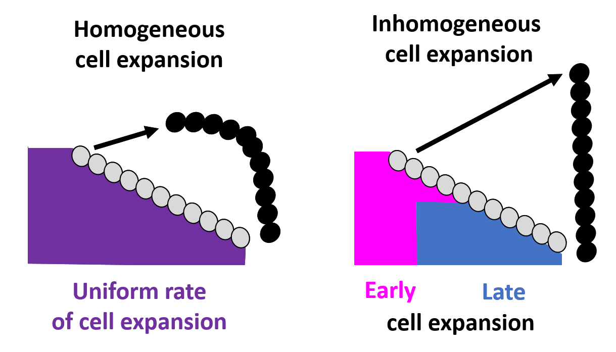
A picture of sex comb rotation finally emerges as a result of this computational-experimental approach. The picture clearly depicts how the underlying epithelial cell dynamics facilitate sex comb rotation—by utilizing the asymmetry in the timing and location of cell growth. First, the epithelial cells start out smaller closer to the leading tip of the comb as compared to the comb base, thus creating an inhomogeneity in initial cell size distribution (Fig. 6).
Figure 6. Homogeneous and inhomogeneous cell growth. Initial (gray circles) and final (black circles) sex comb position. For details, see the primary paper.
As the cells expand, this inhomogeneity translates into a differential push which maintains the shape of the comb during the entire rotation. In addition, the mathematical model identified a temporal component in which delayed expansion of distal cells closer to the comb base protects the combs from breaking during rotation, a phenomenon also subsequently verified by experimental imaging data.
We will discuss below how our discoveries have shed light on the essential relationship between comb evolution and its underlying cellular processes.
Evolutionary implications
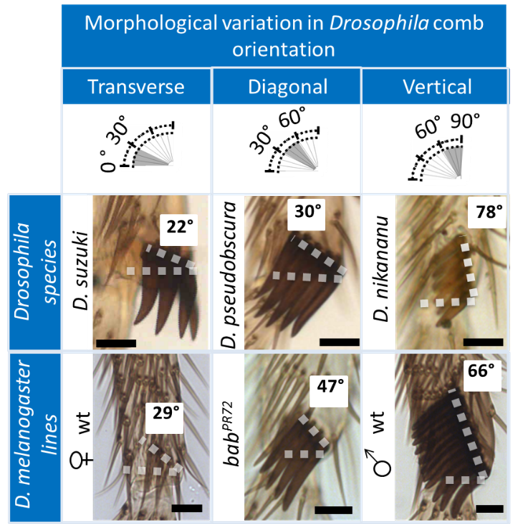
How to modify comb orientation. Sex combs in the family Drosophilidae can be divided into three main groups based on their orientation relative to the joint: transverse (0˚-30˚), diagonal (30˚-60˚), and vertical (60˚-90˚) (Fig. 7).
Figure 7.Morphological variation in Drosophila comb orientation. Adult sex combs of Drosophila species (top panel) and D. melanogaster lines (bottom panels). White dotted line indicates sex comb or bristle row angle relative to the joint. Scale bar:20 µm. D. melanogaster females lack sex combs and are used as a control. For details, see the primary paper.
Phylogenetic analyses reveal that changes in comb orientation not only occur frequently, but also occur between closely related Drosophila species. To study how comb orientation evolves, we used genetic perturbations in D. melanogaster that phenocopy the morphological variations in nature (Mov. 2 and Fig. 7).
Movie 2. Time-lapse movies of D. melanogaster lines with three comb orientations.
In vivo experiments show that a reduction in apical cell expansion leads to a reduction in the angle of rotation. With computer simulations, we now understand that nature exploits the asymmetry of distal cell expansion to achieve this goal. In other words, the smaller the degree of rotation, the smaller the degree the inhomogeneity in cell expansion is required for the rotation. These findings suggest that changes in comb orientation can occur via fine-tuning the pattern of cell growth to achieve the pattern of inhomogeneity we have described. This narrows our focus to determining those genes and tissue forces involved, which will go far in understanding the enigma of sex comb rotation and perhaps other morphogenetic events where local differential growth occurs.
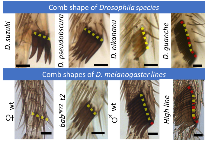
Relationship between comb length and shape. Despite the spectacular morphological diversity observed in Drosophila combs, their shape tends to be straight (Fig. 8).
Figure 8. Morphological variation in Drosophila comb and bristle row shape. Yellow dotted lines indicate sex comb straight shape, while red dotted line show minor bends. Scale bar:20 µm. For details, see the primary paper.
Since the combs are used as a grasping tool, a straight comb shape seems to be fundamental for proper functioning. Our computational model uncovers the critical mechanisms that maintain the comb shape during the entire rotation.
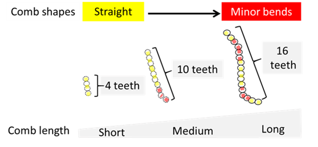
Experimentally, short combs tend to be straight while long combs are more likely to display minor bends (Fig. 9).
Figure 9. Long combs are more likely to bend during rotation. Yellow dotted lines indicate straight sex comb shape, while red dotted lines show minor bends.
In fact, computer simulations show that increasing comb length is associated with multiple mechanical limitations to achieve a proper rotation. Long combs, for instance, are more likely to break during rotation (Mov. 3).
Movie 3. Long combs are more likely to break during morphogenesis. Examples of adult legs displaying sex comb breaking in Drosophila species (A) and Drosophila melanogaster lines (B). Schematic (C) and computer simulation (D) showing sex comb breaking during rotation.
These findings are consistent with the Drosophila comb diversity observed in nature. Most of the long combs (>15 bristles) display a different mechanism to achieve a vertical position. The only exception is Drosophila guanche, but as predicted by our model, this Drosophila comb generally displays bent and broken phenotypes.
Future directions. This work shows that the computational-experimental approach is an effective method to study morphogenesis and its evolution. For example, we can use simulations to further explore the thresholds beyond which long combs are unable to rotate due a spatial limitation1. The computer simulations on sex comb rotation generated many hypotheses that will be tested by combinations of new techniques.
Acknowledgements. We are deeply grateful to Joel Atallah, Lewis Held and Artyom Kopp for their detailed and constructive comments during this challenging project.
Juan N. Malagon is currently a Research Associate with Dr. Ellen Larsen
and hopes to get a faculty position, which allows him to combine his
two passions: teaching and developing research projects with students. His professional website is: https://juannicolasmalagon.com.
The successful applicant will be involved in research and contribute to operations in the area of Genetics and Evolution of Morphogenesis under the direction of the Director Prof. Miltos Tsiantis.
We are seeking an individual with a PhD in biology or a related discipline and demonstrable high-level competence in analysis of morphogenesis and its genetic control, using advanced imaging. Excellent interpersonal and organizational skills are required including outstanding record keeping, good IT literacy, willingness and ability to learn new methodologies and strong communication skills. A key responsibility of the post is to apply and improve advanced imaging methods (e.g. time-lapse imaging). The scientific questions asked relate to how developmental genes regulate cellular growth to generate diversity. Please, refer to Vlad et al. 2014, Science; Rast-Somssich et al. 2015, Genes Dev; Vuolo et al. 2016, Genes Dev; Vuolo et al. 2018, Genes Dev, for relevant published work by the group.
The post holder should also be interested in science management as he/she will contribute to maintaining genetic resources relating to microscopy. The successful applicant will be a strong team player and highly solution-oriented. Payment and benefits will depend on age and experience and will be according to the German TVöD scale for a part-time, 50% position. An appointment will only be made if and when a suitable candidate is identified and applications will be first evaluated end of December. Only shortlisted candidates will be contacted. The post is initially for 2 years with possibility for renewal. The post would suit a young researcher who is passionate about developmental biology and also wishes to obtain training and experience in project management.
The application should include a two-page CV and a letter of motivation stating clearly how previous experience and interests match the post requirements and career aspirations, names and addresses of two referees and should be submitted electronically as one file (yourname_imaging) to Dr. Karakasilioti (applications.tsiantis@mpipz.mpg.de), by 20 December 2018.
The Max-Planck Society is committed to increasing the number of individuals with disabilities in its workforce and therefore encourages applications from such qualified individuals. Furthermore, the Max Planck Society seeks to increase the number of women in those areas where they are underrepresented and therefore explicitly encourages women to apply.
The Max Planck Institute for Plant Breeding Research (MPIZ) in Cologne (http://www.mpipz.mpg.de/2169/en) is one of the world’s premier sites committed to basic research and training in plant science. The institute has four science departments, three independent research groups and specialist support, totaling 400 staff including externally funded positions.
The department of Comparative Development and Genetics at the Max Planck Institute for Plant Breeding Research (MPIZ) is seeking a
Plant Developmental Biologist
The successful applicant will be involved in research and contribute to operations in the area of Genetics and Evolution of Morphogenesis under the direction of the Director Prof. Miltos Tsiantis.
We are seeking an individual with a PhD in biology or a related discipline and demonstrable high-level competence in analysis of morphogenesis and its genetic control, using advanced imaging and genetics. Excellent interpersonal and organisational skills are required including outstanding record keeping, good IT literacy, willingness and ability to learn new methodologies and strong communication skills, including demonstrable ability to write clearly and concisely in English. A key responsibility of the post is to develop and improve advanced developmental biology methods (e.g. time-lapse imaging and use and improvement of methods for analyzing genetic mosaics) and associated approaches. The scientific questions asked relate to how developmental genes regulate cellular growth to generate diversity. Please, refer to Vlad et al. 2014, Science; Rast-Somssich et al. 2015, Genes Dev; Vuolo et al. 2016, Genes Dev; Vuolo et al. 2018, Genes Dev or http://www.mpipz.mpg.de/226344/tsiantis-dpt for relevant published work by the group
The post holder should also be interested in project management as he/she will also contribute to maintaining relevant departmental technical expertise and genetic resources and in training of new or junior researchers. The successful applicant will be a strong team player, highly solution-oriented and will have a key role in ensuring smooth running of lab activities in the area of morphogenesis. He/She will also support funding applications in the area of plant development. Payment and benefits will depend on age and experience and will be according to the German TVöD scale. An appointment will only be made if and when a suitable candidate is identified and applications will be first evaluated end of December. Only shortlisted candidates will be contacted. The post is initially for 2 years with possibility for renewal. The post would suit a young researcher who is passionate about plant developmental biology and also wishes to obtain training and experience in project management.
The application should include a two-page CV and a letter of motivation stating clearly how previous experience and interests match the post requirements and career aspirations, names and addresses of two referees and should be submitted electronically as one file (yourname_devbio) to Dr. Karakasilioti (applications.tsiantis@mpipz.mpg.de), by 20 December 2018.
The Max-Planck Society is committed to increasing the number of individuals with disabilities in its workforce and therefore encourages applications from such qualified individuals. Furthermore, the Max Planck Society seeks to increase the number of women in those areas where they are underrepresented and therefore explicitly encourages women to apply.
The Max Planck Institute for Plant Breeding Research (MPIZ) in Cologne (http://www.mpipz.mpg.de/2169/en) is one of the world’s premier sites committed to basic research and training in plant science. The institute has four science departments, three independent research groups and specialist support, totaling 400 staff including externally funded positions.
 (1 votes)
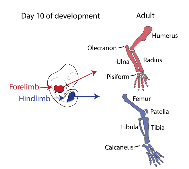
 (No Ratings Yet)


 (4 votes)