A postdoctoral position is immediately available or on the date upon mutual agreement in the laboratory of Jianlong Wang, Ph.D., Department of Cell, Developmental and Regenerative Biology, Black Family Stem Cell Institute, Icahn School of Medicine at Mount Sinai, New York, NY 10029. The position is funded for the study of biochemical basis and regulatory circuitry for totipotent and pluripotent stem cells in the mouse and human, focusing on transcriptional, post-transcriptional and epigenetic mechanisms. Our studies utilize both in vivo mouse and in vitro cell culture models (please refer to our lab research profile here http://www.stemcellwanglab.com). Applicants should have a Ph.D. and/or an M.D. degree and have experience in mouse/human ES cell culture and/or other mammalian cell cultures including cancer cell lines. Prior experience working with laboratory mice, protein biochemistry, and cancer and stem cell biology is beneficial. Knowledge and practical skills on basic bioinformatics such as RNA-seq, ChIP-seq and CLIP-seq data analyses will be a plus.
Our group is part of the Black Family Stem Cell Institute, the MINDICH Child Health Institute and the Tisch Cancer Institute. This highly productive and collaborative environment will provide excellent resources, mentorship and support. The position offers competitive salary, guaranteed subsidized postdoc-housing and exposure to a rich environment at Icahn School of Medicine at Mount Sinai and the New York City/Manhattan area. Interested candidates should send a Cover Letter together with CV and names/contact information of 3 potential references to Jianlong Wang, Ph.D. (jianlong.wang@mssm.edu).
We are still looking for a Scientific Reviews Editor for the journal Development – for full details, please see the job advert here.
You may have noticed that this is not the first time we’ve posted this job. While we would ideally be hoping to recruit someone with some previous editorial experience, we don’t want to put off other candidates; in fact, most Reviews Editors at The Company of Biologists join us straight from the lab, with no direct experience. This is a fantastic opportunity for a developmental biologist (or someone working in a related field) who does not want to continue in the lab, but would like to stay close to the cutting edge of science, and the scientific community – and we are keen to recruit as soon as possible.
If you are interested in this position, please don’t hesitate to get in touch with me (Katherine Brown, the journal’s Executive Editor) if you want an informal chat before applying formally. And if you have any queries about potential eligibility, please get in touch with our HR department.
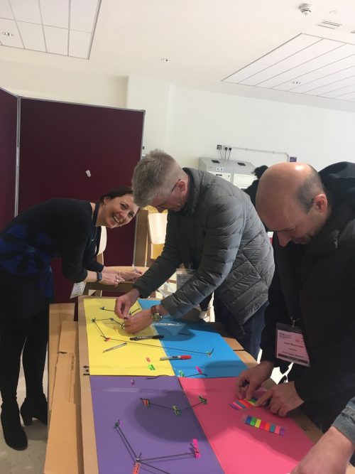
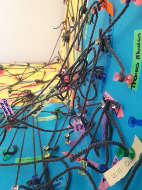
The great and the good of British developmental biology were in attendance, including many BSDB past-presidents and committee members, and, presumably inspired by this historical ambience, the organisers decided to set up a family tree in the atrium. Attendees would put their own names on the board, then those of their PhD and postdoctoral advisers, and link them with string. These details were also taken down on paper.
It started off relatively clean and tidy…
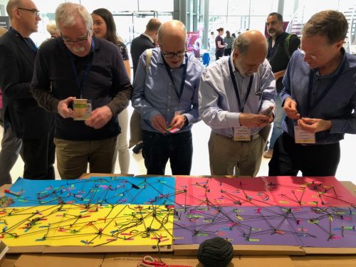
…but as more and more attendees added their details it turned into quite a dense network…
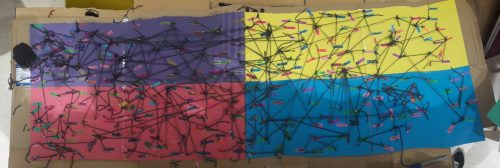
…and by the end of the conference there were hundreds of nodes and edges. The question then came up of what we were going to do with it.
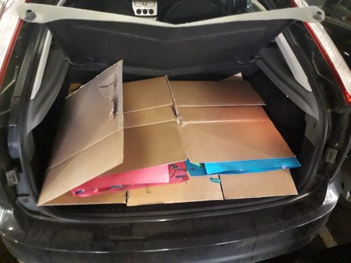
To the delight of the organisers we decided to take the thing back with us to our office in Cambridge. It just about made it into the boot of the car…
…but some the edges and nodes of the network did not prove robust enough to survive the transit in tact (luckily we had the back up sign up sheets).
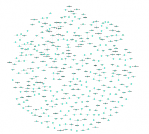
So now it needed digitising. I first just entered the data into Excel – it ended up with 349 connections from individuals to their advisers. There were almost certainly errors in transcription from scribbled handwriting to computer screen but I think I got most connections right.
But the visualisation was less easy to figure out. We could have tried something like Neurotree – The Neuroscience Academic Family Tree, but this didn’t really fit with the network created in Warwick. During my postdoc I had played around with Cytoscapeto visualise protein protein interaction data and this seemed like a better way forward. But I figured though the best thing would be an online tool where no one has to download anything, and stumbled upon Cell Maps – Systems Biology Visualisation.
This site pretty much does what I wanted. You end up with a network that looks like this
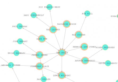
And in close up…
The arrows point to the advisers (hence Jim Smith pointing to Lewis Wolpert and Jonathan Slack, and being pointed at in turn by his students and postdocs!).
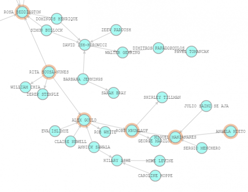
It can be quite fun to follow connections – linking Angelo Nieto to Rosa Beddington, for instance.
How to view the network
You can view and play around with the network yourself – first download this file
And go to http://cellmaps.babelomics.org/, select ‘Open Session’, and load up the file. There’s a search bar – use all caps, full name. And you can also play around with some wacky network layouts (though I think the ‘Force Directed – Default’ setting works the best!).
Any ideas?
There are some issues with this site – I keep on getting errors when trying to export the network as an image, for instance. It’s also not linked with the data itself (I had to turn the Excel into a txt file). So if anyone has other ideas about how to visualise a network of scientific connections, please comment below! Of particularly interest would be ways of visualising extra bits of information in the network (e.g. model organism, nationality, where or when one got their PhD, etc). I really have little idea what I’m doing…
Community curation needed!
One other issue is the data itself, which is clearly incomplete (just look at the single connections of luminaries like Phil Ingham and Angela Nieto!).
So we need further community curation! I’ve put the data from the sign up sheets into a Google Sheets doc. Sheet 1 has ‘raw’ data – the person in question and all of their advisers. Sheet 2 has each interaction, one after the other, which is used as the input into Cell Maps.
You can access the sheet here– and if you were at the meeting but didn’t manage to add to the physical network, I’d appreciate your input!
We’re initially planning to stick just to BSDB attendees, but there’s no reason why we can’t expand this to the global family of developmental biologists. I’d love to know your thoughts on how best to carry this family network forward.
Parasitic plants are fascinating and agriculturally relevant organisms that rely for their success on the haustorium, a specialised root structure that invades host root vasculature to derive nutrients and water. A recent paper in Development addresses the developmental origins of these crucial structures in the facultative root parasite Phtheirospermum japonicum. We caught up with first author Takanori Wakatake and his supervisor Ken Shirasu, Group Director at the RIKEN Center for Sustainable Resource Science in Yokohama, to find out more about the story.
Takanori and Ken
Ken, can you give us your scientific biography and the questions your lab is trying to answer?
KS After I got a bachelor’s degree in agricultural chemistry at the University of Tokyo, I moved to University of California, Davis, where I got a PhD degree in Genetics. My PhD thesis was on how a parasitic bacterial pathogen transfers its DNA to the host plant. As a Postdoc at the Salk Institute, I studied how plant immune signals are potentiated. Then I moved to The Sainsbury Laboratory, UK, where I continued to work on plant immunity identifying signalling components. After nearly 18 years of study abroad, I went back to Japan to open a new lab at RIKEN where I started working on parasitic plants. The main theme of our lab is to understand how plants defend themselves against pathogens and how pathogens overcome it. We work on various pathogens including bacteria, fungi, nematodes and parasitic plants, but often realize that they use similar strategies to manipulate host plants.
Takanori, how did you come to join the Shirasu lab?
TW After I made a decision to study plant science at the graduate school of the University of Tokyo, I was thinking which laboratory I should join. There were two main reasons why I chose Ken’s lab. 1) It is in RIKEN, outside the University of Tokyo. I believed that changing environments would help me to build my identity as a scientist. 2) The term “immunity” sounded cool to me because I was interested in pharmacology when I was an undergrad. I eventually became interested in arms race between plants and pathogen. What Ken suggested to me during the first interview, however, was to study parasitic plants, as pathogens. I decided to work on parasitic plants, because I wanted to do something unique.
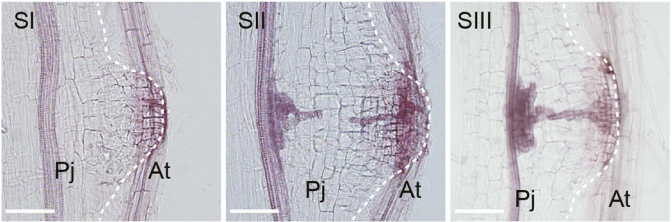
Developmental stages of haustorium formation (Pj, P. japonicum root; At, A. thaliana root), from Figure 1 in the paper.
As far as I can tell, your paper is the first Development has ever published on the development of parasitic plants! What fascinates you about these organisms?
KW & KS How exciting! Parasitic plants are the plants that have evolved to attack own kinds. They do not infect own roots nor members of the same family. Thus, they are able to perceive host plants, which are very similar to themselves, as non-self. How they can differentiate own species from others? And, for infection, they invented a new organ called haustorium, which provides a totally new function. How did plants do that? Haustorium was independently evolved at least 12 times so it should not be so difficult. They must have modified a common machinery so following developmental stages of haustorium we may find some clues.
Time-lapse observation of nuclear behavior during early haustorium development, and with nuclei tracked. From movies 1 and 2 from the paper
Can you give us the key results of the paper in a paragraph?
KW & KS In the paper, we demonstrate that cells in the various layers of the root tissues are reprogrammed and collectively establish a new organ upon host perception. In particular, epidermal cells differentiate into specialized cells to penetrate host tissues. Other various cell types differentiate into vascular meristem-like cells to pave the way to connect parasite vascular and host vascular system for nutrient transfer. This is quite different from known developmental processes such as lateral root and nodule formation. This work also represents a high plasticity of plant roots.
Have you got any ideas about the pathways by which the inductive signals control cell fate transitions in a localised manner in the parasitic root?
KW & KS We are currently working on a putative HIF receptor we identified. We aim to elucidate the signalling pathway from HIF perception to local induction of the YUC3 gene, which encodes a key auxin biosynthesis enzyme to initiate haustorium development.
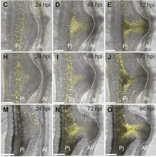
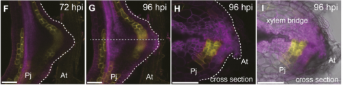
Putative procambium gene expression in the haustorium, from Figure 3 in the paper
Does your work have any implications for how to combat parasitic plants in agriculture?
KW & KS Not immediately. However, once we understand how haustoria are made, we may be able to block the process. Thus, our work set the fundamental base for the future study to dissect the process.
When doing the research, did you have any particular result or eureka moment that has stuck with you?
KW My favourite experiment in the paper is the lineage tracing using the CRE-Lox system. Initially I thought, based on marker analysis, that various cell types actually change cell fate and differentiate into procambium-like cells. To demonstrate this possibility clearly, I needed a lineage tracing experiment during haustorium development. I designed the CRE-Lox system and made a number of constructs. After many trials, I finally got the result indicating that cortex layers differentiate to procambium-like cells. It was a very satisfying moment.
Tracing cell lineage in the haustorium, from Figure 5 in the paper
And what about the flipside: any moments of frustration or despair?
TW At first, I envied the researchers who work on the established model organisms. They can easily access to mutant collections, transformation lines, complete genomes, etc, but now I am fine with our situation and try to think about what we can do. I believe new technologies such as CRISPR and magnetfection will drive the research in non-model plants.
What next for you after this paper?
TW Currently, I am trying to wrap up another paper about auxin flow and xylem bridge formation in the haustorium. After that, I would like to challenge in a new research field.
And where will this work take the Shirasu lab?
KS Intrusive cells are the interface between the parasite and host. They need to deal with host immunity system and find location of host xylem. There must be many signals going by between parasites and hosts. We aim to identify those signals.
Finally, let’s move outside the lab – what do you like to do in your spare time?
TW In general, I like listening nice music, playing games, and watching football games. Recently, I am into watching films and learning cinematography. I am also studying spices for cooking.
KS I enjoy cooking at home. I think that cooking is a creative experience, which makes me excited. It’s more like planning and doing experiments, and at the same time I can feed my family! Vegetables are coming from my small vegetable garden, where I combat a lot of pathogens! So I can do some plant immunity studies there, too!
It’s hard to describe with words how my experience has been at the Marine Biological Laboratory (MBL) in Woods Hole, Massachusetts, but I’m going to give it a try…
My attendance at the 2018 Embryology course at the MBL, has been possible thanks to an award I won in my home country, during the International course on Developmental Biology, held in Quintay, Chile (a post written by the students of the course was published before https://thenode.biologists.com/tracing-the-origins-of-developmental-biology-in-latin-america/events/ ). I felt incredibly fortunate at the time to be considered to participate in this lifechanging experience at the MBL, but it wasn’t until now that I understood what it really meant.
Performing research in Chile, as well as in most Latin American countries is quite challenging, both in terms of funding, equipment availability and time (imported items take at least one or two months to arrive). We are forced to learn how to plan experiments with caution, which is in part great as we become efficient with scarce resources (but also terrible because it limits our scientific creativity).
Here at the MBL it is the exact opposite: I can be the “crazy scientist” that I have always dreamed about, by not only repeating classical embryological experiments in all sort of species, but also thinking outside the box and testing new hypotheses without the fear of failure. This is one of the things that I’ve loved the most about the course.
I have been incredibly lucky to be able to work with so many different species, image them with a huge variety of microscopes (seriously, so many!) and yet, still had to struggle to get a slot because we were all so eager to use them. We learned how to make our own tools with Walmart items and to forge instruments with three different flames. We also had the opportunity to perform novel techniques, such as in utero CRISPR editing of mice and single molecule in situ hybridization in arthropods, among others.
Collecting samples at the MBL and field use of Foldscope with its creator Manu Prakash
And obviously, I’m aware that our lecturers are leaders in their fields from around the world. I enjoy hearing about and discussing their work first hand, as well as having the time to interact with them personally over lunch or dinner. I remember the wonderful talk that we had the privilege to witness, given by Nobel Laureate Eric Wieschaus about the biophysical properties of Drosophila development. During our famous “sweatbox” (intense Q&A), we got the opportunity to gain further insight into his mind. Someone in the audience asked how he dealt with failure, to which he smartly replied “well, failing I’m used to, so I consider myself an expert by now”, which provoked a general laughter in the room, as we all know that experimental fiascos are a common problem in our field. But he then added sage advice to that initial comment – celebrate every small success, and don’t allow every failure to discourage you.
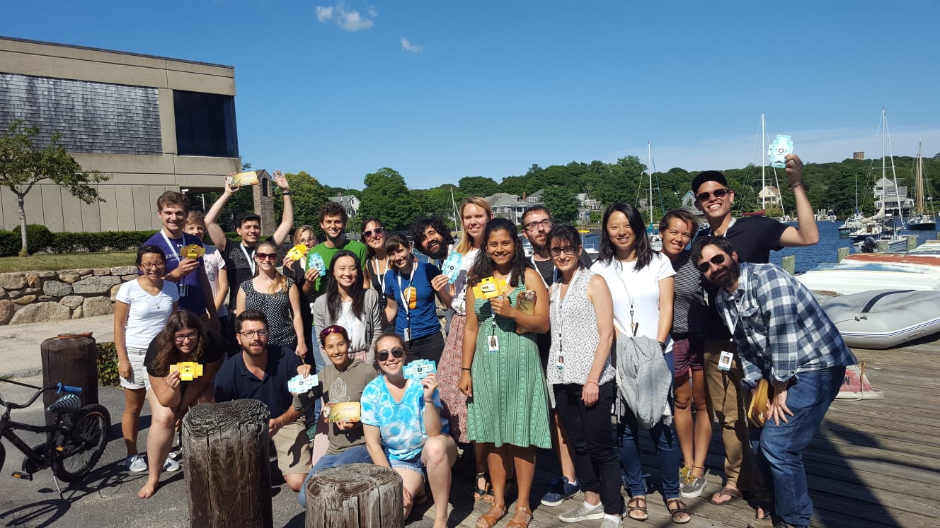
Apart from the top scientific and intellectual level of all attendees, the people I have met are incredible, coming all from different backgrounds and cultures and I’ve learned so much from all of them. I really like the bonds that have been established amongst our group. We all contribute with our knowledge and skills, whether it was during lectures, bench work, microscope use, and even during softball practice. Of course, I’ve also enjoyed sharing a beer in our break room or at the Kidd, as well as eating in Pie in the Sky and going to the beach “collecting samples”. I have no doubt that this group will stay in touch and even collaborate in the future. I’ve been here for almost 6 weeks now and it’s been exhausting, a level of sleep deprivation that I thought I was incapable of handling at my almost 30 years old, but totally worth it.
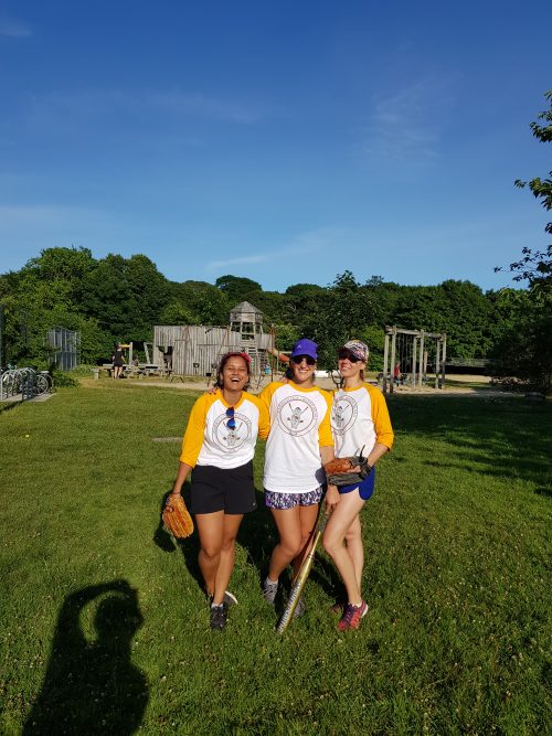
After winning the famous softball game, with my friends Aastha and Martyna
Two days before the end of it, I’m ready to go back to the real world, but a part of me never wants this experience to end. Overall, having attended the 2018 MBL Embryology course has changed my life, and I am so glad it did. For whoever is reading this article, I encourage you to apply for the 2019 class, I promise that it will also change yours…
Asymmetric division is a widespread mechanism for generating cellular diversity during developmental patterning. The stomata of flowering plants are epidermal valves that regulate gas exchange, and provide an accessible system to investigate the mechanisms of asymmetric cell division both within and across species. A paper in the new issue of Development reports an investigation of the molecular control of this process during development in the forage grass Brachypodium distachyon. We caught up with co-first author Ximena Anleu Gil and her supervisor Dominique Bergmann, Professor of Biology at Stanford University, to hear more about the story.
Ximena and Dominique
Dominique, can you give us your scientific biography and the questions your lab is trying to answer?
DB I’ve been fascinated by development, and especially the relationship between asymmetric cell division and cell fate, for more than two decades. As a PhD student, this meant studying body axis formation in C. elegans. I still love the stunning microscopy possible with worm embryos, but I began to be interested in less invariant development—we know most organisms have some degree of flexibility (and uncertainty) in their developmental trajectories– and so, as postdoc, I moved to plants to ask about the relationships between cell polarity, asymmetric divisions, and cell identity in organisms with a great deal of plasticity, resilience, and environmental responsiveness.
The challenge, of course, in choosing to work on something with flexible development is that to have any hope of dissecting genetic networks or organizing principles you need to focus on some relatively simple decisions. For my lab, that has been the development of stomata (pores that mediate uptake of CO2 from the atmosphere in exchange for water vapor from the plant) in the epidermis of leaves. Most of the lab works on stomata in Arabidopsis, where stomata and their non-stomatal neighbors are the product of a simple epidermal lineage: we are fascinated by the stem cell-like asymmetric divisions at the beginning of this lineage that can be modulated to create leaves of different sizes with different numbers of stomata. These days, we are looking at the lineage through transcriptomic and epigenomic approaches, by developing imaging tools to monitor asymmetric divisions and also by collaborating with ecophysiologists to look at how development affects behaviors in the “real world” and vice versa.
Ximena, how did you come to join the Bergmann lab, and what drives your research?
MXAG I joined the Bergmann lab as a lab technician after I finished my college degree. I had been studying the heat shock response mechanism in plants and was looking for technician jobs in other plant labs to expand my lab skills and also experience real-life science before starting a graduate degree. I was extremely lucky because Dominique was looking for a technician at that time.
I define and re-define my motivations as I learn more about the incredibly complex and beautiful world of biology, but what never changes is my amazement with the natural world. Visually and intellectually, nature is a fascinating puzzle to try to decipher. And as I learn more about plants and their flexible but robust development, I have become deeply intrigued with trying to understand developmental decisions from a plant’s perspective. The plant kingdom is so diverse and important for our planet and society, I feel that we should spend more time thinking about it.
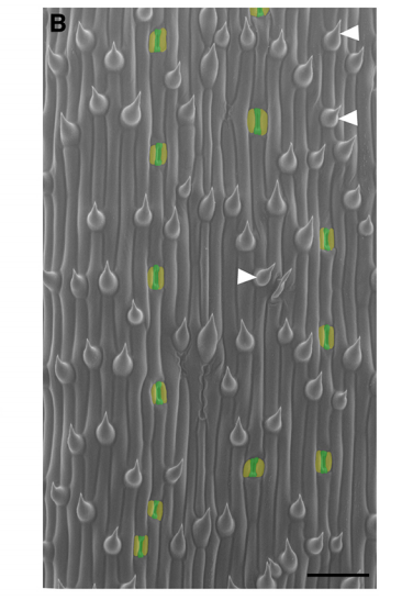
SEM of wild type Brachypodium epidermis, with guard cells in green, subsidiary cells in yellow, arrows showing co-existence of stromatal and hair fates in a single file. From Figure 1 in the paper
What makes Brachypodium a good (comparative) model for asymmetric cell division in development, and what were the gaps in your knowledge about the process before your current work?
DB & MXAG The stomatal lineage of Brachypodium, like those of rice, maize, wheat, and other grasses, is very organized. You can think of its development as a time-line where spatial position (base vs. tip of leaf) is a proxy for time. It’s like the Arabidopsis root in this way, which lends itself to certain simplifying behaviors relative to the randomly oriented self-renewing divisions of Arabidopsis. When YODA, the kinase at the heart of our recent Development paper, was first characterized, it was in the context of asymmetric divisions in the Arabidopsis embryo (by Wolfgang Lukowitz and colleagues) and the stomatal lineage. From these early studies, it was thought that the processes of physically asymmetric division and establishment of different cellular fates were intrinsically linked, and both controlled by YODA. Neither the Arabidopsis embryo (tiny and inaccessible for long-term imaging) nor the stomatal lineage (with its rounds of asymmetric division) could give us much clarity on the real connection between a physically asymmetric division and its immediate fate outcome. The beautifully ordered epidermis of Brachypodium allowed us to study them separately, both conceptually and experimentally. The presence of epidermal cell types not present in Arabidopsis like hairs and silica cells also gave us new things to measure, and it was exciting (but unexpected) that their patterning would also controlled by YODA. Finally, not inconsequentially, as challenging as it was to analyze the dwarfed bdyda1 mutants, atyda would have been worse because the plant is even tinier!
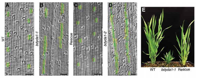
DIC images of Brachypodium abaxial epidermis and whole plant phenotypes, from Figure 2 in the paper
Can you give us the key results of the paper in a paragraph?
DB & MXAG Asymmetric cell divisions are feature of plants, animals and microbes and, in multicellular organisms, are critical to establish pattern and cell-type diversity. Much of our thinking about asymmetric divisions comes from flies and worms, where ideas about creating physical asymmetries and orienting the division of a mother cell has direct consequences for fate (through segregation of fate determinants or positioning of daughters near instructive cues). In our paper, we report the identification and characterization of a mutant isolated from a forward genetic screen based on its production of clustered stomata—typically a readout for defects in cell fate and asymmetric division. Through complementation experiments and CRISPR/Cas9 genome editing, we confirmed that the phenotypes were caused by mutations in the BdYDA1 gene. BdYDA1 is a very close homolog of AtYDA MAPKKK gene, a crucial member of a MAPK signalling cascade that is required to inhibit stomatal cell fate and enforce a patterning rule that prevents stomata from being direct neighbors in Arabidopsis. In contrast to loss of the Arabidopsis counterpart, bdyda1 mutants also displayed the same patterning defects in other non-stomata epidermal cells, including hair cells and silica cells. Surprisingly, each of these clustered patterns did not seem to arise from faulty physical asymmetric cell divisions but from improper enforcement of alternative cellular fates in these tissues. Our phenotypic analysis suggests that in Brachypodium, BdYDA1 works as part of a general molecular switch that controls cell identity to ensure proper spacing of epidermal cell types. They also helped expand our understanding of the mechanisms through which YODA genes are acting in the establishment of differential cell fates during plant development.
In terms of its upstream and downstream factors/signalling cassettes, how similar do you think BdYDA1 works compared to AtYDA?
DB & MXAG We have no reason to think that kinase activity differs between AtYDA and BdYDA1, however, each of these proteins has a large, less well conserved, N-terminal domain. In Arabidopsis, this domain regulates protein activity and is suspected to link AtYDA to upstream kinases, one of which has unique features in the Brassicas (mustard plant family, including Arabidopsis), so that suggests potentially different upstream inputs. On the other hand, homologues of the EPF family of signaling peptides that act upstream of AtYDA are found in grasses and overexpression of one of these in barley affects stomata (Hughes et al., 2017 doi.org/10.1104/pp.16.01844) so there is some potential for conservation, too.
Downstream, work in Arabidopsis revealed a core set of dedicated stomatal transcription factors that promote the entry into, and exit out of stem-cell like divisions, as well as guide the differentiation process of stomatal guard cells. The expression and protein stability of these transcription factors are highly regulated, and about a decade ago Ph.D. student Cora MacAlister and postdoc Greg Lampard found that the stomatal initiating factor SPEECHLESS (so named for the absence of stomata or “mouths”) was phosphorylated by MAPKs downstream of YODA. SPCH has been duplicated in Brachypodium and neither paralog encodes a protein with all the known MAPK sites present in AtSPCH, so it is possible that the BdSPCHs aren’t the ultimate target of BdYDA1. And we certainly have no idea what the targets in silica and hair cells might be! What is also really interesting is that homologues of the Arabidopsis polarity protein BASL, which is both target of MAPK phosphorylation and potential scaffold enabling differential AtYDA inheritance after asymmetric division, are not found at all in grasses. What, if anything, is used in BASL’s place?
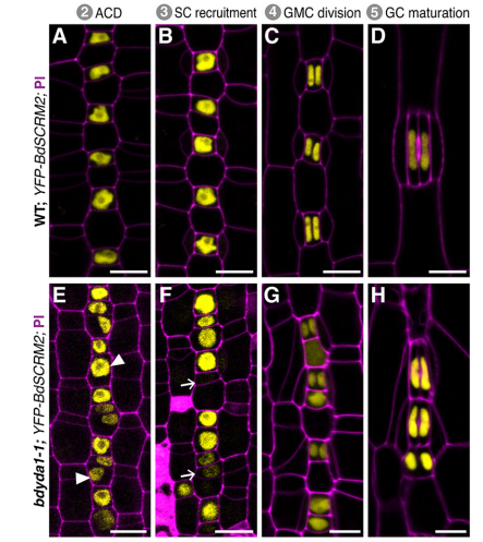
Stomatal development in Brachypodium, from Figure 4 in the paper
What does this work tell you more broadly about how cell fates are determined in plants?
DB & MXAG Unlike animal development, plant development mostly occurs post-embryonically and is heavily influenced by the environment. The Arabidopsis stomatal lineage for example, has the flexibility to modify the number of precursor cells in response to their environment, and it does so by regulating the number and types of asymmetric divisions. Environment can also mean “neighbor cells” and more and more evidence is accumulating from root development and grass stomatal subsidiary cell recruitment (Raissig et al., 2017, doi:10.1126/science.aal3254) that neighboring cells have a stronger role in providing the appropriate signals that determine cell fate. There are more questions than answers now, but our BdYDA1 work sheds some light into some of these inquiries. We propose a shift in our understanding of MAPK signaling during asymmetric cell division in plants, from being all about the physical asymmetry of cells before and after a division event to thinking about this process as a more dynamic one, i.e. one that requires enduring cross-talk between neighboring cells to ensure the correct fate of daughter cells after an asymmetric division event. Our thinking is that plant cells are locked in place and there is no programmed death and removal of cells; thus, what a cell becomes is of great significance to neighbors stuck beside it for life—it’s in the interest of these neighbors to provide cues to coax that cell into becoming something appropriate, and for that cell to take its time evaluating the incoming information.
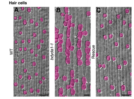
Brachypodium leaf epidermis with hair cells false-colored magenta, from Figure 5 in the paper
When doing the research, did you have any particular result or eureka moment that has stuck with you?
MXAG A BdYDA1 allele was identified in a screen that Emily Abrash and Juliana Matos (with Akhila Bettadapur) initiated back in 2011, and BdYDA1 was actually the first Brachypodium gene Emily cloned, using a “clone by guessing” strategy—the plant phenotypes of excessive stomata and compact growth were so reminiscent of AtYDA mutants that a homologue seemed like an obvious choice. But after Emily confirmed that she had a mutation in BdYDA1, the project was put on the back burner for a while because the phenotypes were so superficially similar in atyda and bdyda1 mutants that we doubted we’d learn anything new. It wasn’t until we created the cell identity markers (BdSPCH2-YFP, BdMUTE-YFP and BdSCRM2-YFP) and tools for live cell imaging that it became clear that something was different! I was tasked with finishing this project started by the original Brachy team, and at the beginning was a little nervous about re-analyzing Emily’s data and re-evaluating her interpretations. I spent a lot of time in the microscope looking at the epidermis of WT and bdyda1 plants and developed a feeling that asymmetric cell divisions looked just fine in bdyda1. But, since this observation ran counter to the dogma in the field, initially I didn’t feel so confident about my observations, nor did I fully understand the implications this would have for our understanding of stomatal development. After many, many meetings with Dominique and other lab members, presenting in lab meeting, attending conferences, and finally putting this project in paper format, I gained confidence. Then things just came full circle! I wouldn’t say it was a eureka moment because I had to convince myself and others that what I was observing was real and reproducible.
And what about the flipside: any moments of frustration or despair?
MXAG Of course! My self-confidence was shaken quite a bit during this time… worries that I was being too slow doing experiments, reading relevant papers, writing the paper, etc. I had done research as an undergrad and had had my own projects, but nothing of this magnitude. I had to learn many, many things like taking breaks, balancing my time working independently with my role as technician, and re-motivating myself when academic science felt too far away from the real world, among other things. I couldn’t have done it without such a supportive PI and lab. I was extremely lucky to have friends who reminded me about the importance of taking care of myself and having fun while doing research! More concretely, working with bdyda1 is quite difficult. The plants are so small and they don’t always want to be photographed… so trying and trying until I got the picture I needed and wanted without a doubt tested my patience and diligence.
What next for you after this paper?
MXAG I’m extremely excited to start my PhD! I’ll be joining the Plant Biology group at UC Davis where I hope to continue exploring plant development.
And where will this work take the Bergmann lab?
DB The initial idea for moving to Brachypodium was to use genetic screens to probe novelties in the grass stomatal lineage, like the rigid, file-like organization of stomata and their precursors and the presence of subsidiary cells flanking the stomatal guard cells. These screens, however, told us that the massive changes in stomatal form and pattern were due to minor rewiring of the core genetic components (e.g., Raissig et al., 2016 and 2017). This changed my attitude toward the experimental approach and the value of Brachypodium. We are unlikely to do more forward genetic screens, but rather will use Brachypodium (and CRISPR/Cas) to test ideas about conserved or divergent developmental mechanisms. I’m intrigued by a couple of projects we have going that suggest subfunctionalized, or even opposite, roles of Arabidopsis and Brachypodium genes in stomatal development. These studies might give us insight into protein evolution, or might reveal how the different developmental strategies of Arabidopsis and Brachypodium place different demands on the same protein activity. But I’m really excited that while the Bergmann lab may be streamlining its Brachypodium projects, former postdoc Michael Raissig, will be expanding the Brachypodium universe in his own new group at the University of Heidelberg in Germany.
Finally, let’s move outside the lab – what do you like to do in your spare time in California?
DB I love being outside in California, in all its seasons and diverse places: the mountains, the ocean, the forests. It’s magnificent to be out biking and hiking, and also eating and drinking products of this state’s agricultural bounty.
MXAG: I also enjoy spending time outside, particularly going to the ocean. I love the Pacific Northwest coastline because is so peaceful and mesmerizing. I’m also a big foodie! So, cooking, going to restaurants and farmer’s markets, eating… yeah I do a lot of that here.
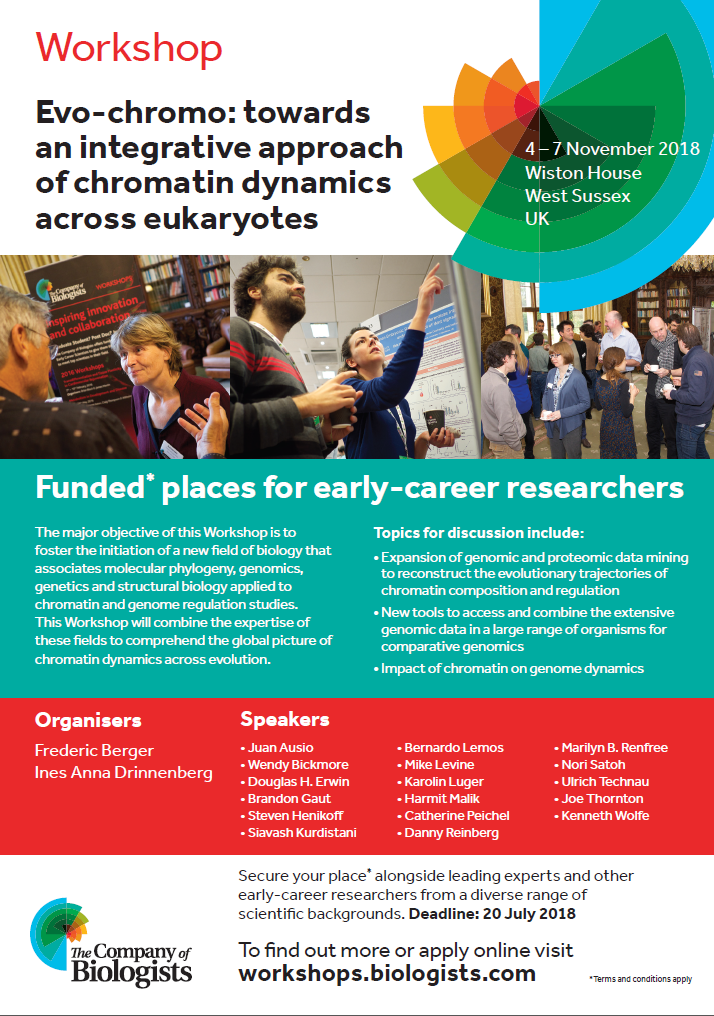
***Deadline to apply for funded ECR places is July 20!***
In November, the Company of Biologists is hosting the latest in its series of Workshops. ‘Evo-chromo’ aims to integrate skills and interests of the fields of chromatin biology and evolutionary biology – if you are an early career researcher and this all sounds appealing to you, the Workshop is currently accepting applications for funded places. Our Community Manager Aidan Maartens will be there – it looks like it will be a fascinating event!
For more information about the Workshop’s scope and aims, and for details about how to apply, visit:
The successful candidate will participate in the cardiovascular research project funded by the BHF, that is in line with the overall objectives of the research group led by Doctor Matthew Stroud at the BHF Centre of Research Excellence, King’s College London (http://bit.ly/stroudlab). The aim of the project is to study the role of the nuclear envelope in cardiac development and disease using a range of molecular, cellular and physiological approaches. We are looking for a highly motivated researcher who possesses strong interpersonal skills with a biomedical background and will pursue collaborative research with members of the team. Furthermore, they will have expertise in cardiac development, physiology, cell biology, molecular biology. He/ she should also be a self-starter and able to work independently, accurately judge priorities, and have excellent organisational and communication skills. Previous experience of relevant techniques such as primary cell isolation and mass spectrometry will be considered highly suitable for this post. Knowledge and experience of integrative cardiac physiology approaches in animal models, such as in vivo cardiac phenotyping and management of gene-modified colonies will also be an advantage.
The BHF Centre of Research Excellence provides an excellent highly multidisciplinary environment with state-of-the-art equipment and facilities. Informal enquiries may be made to: matthew.stroud@kcl.ac.uk.
Developing brains use a mechanism like the Otoshi-buta (the drop lid), a kitchen wisdom.
Differentiating cells in embryonic cerebral walls form a dense filter-like layer to mechanically barrier nuclei of neural stem cells.
Loss of this barrier or fence results in abnormal popping out of neural stem cells’ nuclei, leading to inability of neural stem cells to produce new cells.
Brain formation relies on production of new cells by neural stem cells, which abundantly exist in the embryonic period. Neural stem cells are thin and elongated like radish sprouts (Kaiware-daikon) or Enoki mushrooms. They move their nuclei depending on the status of cell production. They divide along the inner (apical) surface of the wall and their nuclei are therefore near the surface just before and after mitosis, while their nuclei are away from the surface when they synthesize DNA in preparation for subsequent division. The range of this elevator-like (to-and-fro) nuclear movement is about 100μm even though the total length/height of each neural stem cell is ~300μm. Why (for which biological significance) it should be limited and how this range limitation is established are both unknown.
Research Results
In the present study, Professor Takaki Miyata, Assistant Professor Takumi Kawaue, and a 6th year medical student Yuto Watanabe in Nagoya University Graduate School of Medicine (dean: Kenji Kadomatsu, M.D., Ph. D.) showed that a transient layer consisting of differentiating cells and their dense processes mechanically barriers nuclei of neural stem cells. Experimental drilling of this barrier-like layer resulted in abnormal popping out of neural stem cells’ nuclei and the arrest of cell production by such nuclei-overshot stem cells. Thus demonstrated importance of mechanical limitation of nuclear movement during brain development is reminiscent of the usefulness of the Otoshibuta (Drop Lid) to limit a cooking space for condensing soap and avoiding undesired floating of ingredients.
Slides demonstrating the cooking analogy – click to expand
Research Summary and Future Perspective
Boomerangs or artificial satellites should turn back at an appropriate point. This study found that mouse neural stem cells’ nuclei start to come back after a 100-μm going because they are mechanically fenced by differentiating cells there. Drilling of the fence resulted in abnormal popping out of stem cells’ nuclei to 200μm. Since the normal range of nuclear shuttling is much greater in human (200μm), this study provides a basis of future comparative studies aiming at
elucidation of mechanisms underlying evolution of the human brain.
A postdoctoral position is available in the laboratory of Dr. Sophie Astrof at Thomas Jefferson University to study roles of cell-extracellular matrix (ECM) interactions in cardiovascular development and congenital heart disease. We have recently discovered that progenitors within the second heart field (SHF) give rise to endothelial cells composing pharyngeal arch arteries. Projects in the lab focus on the role of ECM in regulating the development of SHF-derived progenitors into endothelial cells and their morphogenesis into blood vessels. The successful candidate will combine genetic manipulation, embryology, cell biology, and confocal imaging to study molecular mechanisms of micro-environmental sensing during vascular development.
Astrof laboratory is a part of a modern and well-equipped Center for Translational Medicine at Jefferson Medical College (http://www.jefferson.edu/university/research/researcher/researcher-faculty/astrof-laboratory.html) located in the heart of Philadelphia.
To apply, please send a letter of interest detailing your expertise, CV and names and contact information of three references to sophie.astrof@gmail.com


 (No Ratings Yet)
 (5 votes)
 (20 votes)